The statistics discussed in this Regional Quarterly Report include the following: (1) advance real state gross domestic product (GDP) statistics for 2017 and revised GDP statistics for 2014–2016, (2) regional price parities and real per capita personal income for 2016, and (3) Arts and Cultural Production Satellite Account statistics for 2015 and updated statistics for 2013 and 2014. For the first time, the Bureau of Economic Analysis included state-level statistics for value added by arts and cultural industries for 2001 to 2015.
Real state GDP grew 2.1 percent on average in 2017, ranging from 4.4 percent in the state of Washington to –0.2 percent in Connecticut and Louisiana according to the advance estimates of GDP by state. Washington’s growth rate accelerated in 2017 from its trend growth rate of 3.3 percent (the average annual percent change from 2011 to 2016). In both periods (2017 and 2011–2016), Washington grew at a faster pace than the nation (table 1) (the average annual growth rate from 2011 to 2016 for the United States was 2.0 percent). Retail trade contributed 1.4 percentage points to Washington’s real GDP growth rate in 2017, and information services contributed 1.0 percentage point. These industries each contributed 0.2 percentage point to growth nationally. California, Florida, Texas, and six other states also grew faster than the nation in both periods.
New York and 26 other states grew slower than the United States in both periods. Notably, the decline in Connecticut’s and Louisiana’s real GDP in 2017 was a continuation of the declines in those states over the previous five years. The finance, management, and state and local government industries in Connecticut reduced real GDP growth in 2017 by 0.8 percentage point. In Louisiana, nondurable goods manufacturing subtracted 0.9 percentage point from real GDP growth.1
Table 1. Real Gross Domestic Product (GDP) by State
[Percent change at annual rates]
| States | 2011 to 2016 | 2016 to 2017 |
|---|---|---|
| Faster than U.S. growth in both 2011–2016 and 2016–2017 | ||
| California | 3.4 | 3.0 |
| Colorado | 3.0 | 3.6 |
| Florida | 2.5 | 2.2 |
| Georgia | 2.4 | 2.7 |
| Idaho | 2.3 | 2.7 |
| South Carolina | 2.1 | 2.3 |
| Tennessee | 2.5 | 2.5 |
| Texas | 3.6 | 2.6 |
| Utah | 3.0 | 3.1 |
| Washington | 3.3 | 4.4 |
| Slower than U.S. growth in both 2011–2016 and 2016–2017 | ||
| Alabama | 0.8 | 1.2 |
| Alaska | −1.6 | 0.2 |
| Arkansas | 1.1 | 1.1 |
| Connecticut | −0.3 | −0.2 |
| Delaware | 0.9 | 1.6 |
| Hawaii | 1.8 | 1.7 |
| Illinois | 1.1 | 1.2 |
| Kansas | 1.2 | −0.1 |
| Kentucky | 0.7 | 1.8 |
| Louisiana | −0.1 | −0.2 |
| Maine | 0.7 | 1.4 |
| Maryland | 1.2 | 1.5 |
| Mississippi | 0.8 | 0.3 |
| Missouri | 0.8 | 1.1 |
| Montana | 1.6 | 0.6 |
| New Hampshire | 1.6 | 1.9 |
| New Jersey | 1.1 | 0.9 |
| New Mexico | 0.6 | 0.8 |
| New York | 1.4 | 1.1 |
| Ohio | 1.6 | 1.9 |
| Pennsylvania | 1.8 | 1.8 |
| Rhode Island | 0.8 | 1.6 |
| South Dakota | 1.0 | 0.3 |
| Vermont | 0.5 | 1.1 |
| Virginia | 0.6 | 2.0 |
| Wisconsin | 1.6 | 1.7 |
| Wyoming | −0.9 | 2.0 |
| Other states | ||
| Arizona | 1.7 | 3.2 |
| Indiana | 1.6 | 2.1 |
| Iowa | 2.8 | 0.5 |
| Massachusetts | 1.7 | 2.6 |
| Michigan | 1.9 | 2.3 |
| Minnesota | 2.0 | 1.9 |
| Nebraska | 2.0 | 0.6 |
| Nevada | 1.4 | 3.5 |
| North Carolina | 1.5 | 2.3 |
| North Dakota | 4.4 | 1.0 |
| Oklahoma | 2.9 | 0.5 |
| Oregon | 0.9 | 2.5 |
| West Virginia | −0.2 | 2.6 |
Note. The United States grew 2.0 percent (2011–2016) and 2.1 percent (2016–2017).
Revised GDP statistics for 2014–2016
The advance state GDP statistics for 2017 are based primarily on the national GDP statistics by industry and BEA estimates of earnings by state and industry.2 Substantially richer state source data are now available for earlier years and have been incorporated in revised GDP statistics for 2014–2016. In addition to a disaggregation by industry, the state GDP statistics for 2014–2016 show the distribution of income from production to labor (compensation), capital (gross operating surplus), and government (taxes on production and imports less subsidies).
Nominal GDP fell in 6 states in 2016—North Dakota (5.2 percent), Oklahoma (4.3 percent), Wyoming (3.9 percent), Alaska (3.6 percent), Louisiana (1.8 percent), and Texas (0.6 percent) (table 2). Real GDP fell in those states as well as in Delaware (1.0 percent), West Virginia (0.8 percent), Connecticut (0.3 percent), and New Mexico (0.1 percent).
In Alaska, taxes on production and imports accounted for almost half of the decline in nominal GDP in 2016 (table 3), reflecting a reduction in tax receipts from the mining industry. In Alaska’s mining industry, taxes on production and imports fell $933 million, gross operating surplus fell $603 million, and compensation of employees fell $514 million in 2016.
In Oklahoma, North Dakota, and Louisiana, in contrast, gross operating surplus accounted for most of the decline in nominal GDP. In Oklahoma, for example, GDP fell $8.1 billion, gross operating surplus fell $6.8 billion, and compensation of employees fell $1.5 billion in 2016. Taxes on production and imports rose $0.2 billion (table 3).
In Texas, compensation grew $10.1 billion and taxes on production and imports rose $3.0 billion in 2016. Nevertheless, nominal GDP fell $10.4 billion because of a $23.4 billion decline in gross operating surplus. In the mining industry alone, gross operating surplus fell $33.5 billion. Texas accounted for 43 percent of U.S. mining GDP in 2016.
The decline in Wyoming’s GDP was accounted for by compensation and gross operating surplus: GDP fell $1.5 billion, compensation fell $0.8 billion, and gross operating surplus fell $0.7 billion; taxes on production and imports less subsidies were essentially unchanged.
Table 2. Gross Domestic Product by State
[Percent change]
| Nominal | Real | |||
|---|---|---|---|---|
| 2015 | 2016 | 2015 | 2016 | |
| United States | 4.0 | 2.8 | 2.7 | 1.5 |
| Alabama | 3.0 | 2.2 | 1.2 | 1.1 |
| Alaska | −9.9 | −3.6 | −1.6 | −3.6 |
| Arizona | 4.4 | 3.8 | 2.1 | 2.0 |
| Arkansas | 1.0 | 1.8 | 0.4 | 1.0 |
| California | 6.4 | 4.4 | 4.6 | 3.0 |
| Colorado | 3.3 | 2.6 | 3.6 | 1.4 |
| Connecticut | 3.6 | 1.4 | 1.1 | −0.3 |
| Delaware | 5.4 | 1.5 | 3.0 | −1.0 |
| District of Columbia | 4.5 | 3.4 | 1.9 | 1.5 |
| Florida | 6.8 | 4.4 | 4.2 | 2.6 |
| Georgia | 5.5 | 5.3 | 3.0 | 3.4 |
| Hawaii | 6.3 | 3.7 | 3.6 | 2.0 |
| Idaho | 3.7 | 4.5 | 2.6 | 3.5 |
| Illinois | 3.6 | 2.4 | 1.2 | 0.9 |
| Indiana | 2.3 | 3.5 | 0.0 | 2.6 |
| Iowa | 5.3 | 3.2 | 3.8 | 2.1 |
| Kansas | 2.2 | 2.1 | 1.4 | 1.7 |
| Kentucky | 2.7 | 2.5 | 0.5 | 1.1 |
| Louisiana | −0.7 | −1.8 | 1.1 | −0.4 |
| Maine | 3.2 | 3.9 | 0.6 | 2.0 |
| Maryland | 4.0 | 4.3 | 1.5 | 2.5 |
| Massachusetts | 6.7 | 3.1 | 4.0 | 1.2 |
| Michigan | 5.6 | 3.5 | 2.6 | 1.9 |
| Minnesota | 2.7 | 3.8 | 0.8 | 2.7 |
| Mississippi | 1.6 | 2.7 | 0.1 | 2.0 |
| Missouri | 3.3 | 1.8 | 0.9 | 0.2 |
| Montana | 2.4 | 0.6 | 2.9 | 0.7 |
| Nebraska | 3.5 | 2.4 | 2.5 | 1.9 |
| Nevada | 6.8 | 4.3 | 4.1 | 2.1 |
| New Hampshire | 5.4 | 3.6 | 2.9 | 2.0 |
| New Jersey | 3.8 | 2.2 | 1.3 | 0.6 |
| New Mexico | −1.7 | 0.3 | 1.6 | −0.1 |
| New York | 4.8 | 2.9 | 2.0 | 0.5 |
| North Carolina | 5.6 | 3.2 | 2.8 | 1.2 |
| North Dakota | −5.5 | −5.2 | −2.5 | −4.9 |
| Ohio | 2.7 | 2.1 | 1.0 | 0.8 |
| Oklahoma | −4.5 | −4.3 | 2.9 | −3.8 |
| Oregon | 6.8 | 5.1 | 4.8 | 3.8 |
| Pennsylvania | 3.5 | 2.0 | 2.6 | 0.9 |
| Rhode Island | 4.6 | 2.3 | 1.9 | 0.5 |
| South Carolina | 6.1 | 4.0 | 3.2 | 2.2 |
| South Dakota | 3.5 | 3.0 | 2.5 | 1.6 |
| Tennessee | 6.2 | 4.7 | 3.3 | 2.8 |
| Texas | −0.1 | −0.6 | 4.4 | −0.4 |
| Utah | 6.0 | 5.3 | 4.2 | 3.3 |
| Vermont | 3.0 | 3.3 | 0.7 | 1.5 |
| Virginia | 4.4 | 2.4 | 1.8 | 0.5 |
| Washington | 6.1 | 5.2 | 3.8 | 3.9 |
| West Virginia | −1.6 | 0.0 | 0.2 | −0.8 |
| Wisconsin | 4.3 | 3.4 | 1.9 | 1.9 |
| Wyoming | −4.9 | −3.9 | 1.2 | −3.4 |
Table 3. Change in State GDP and its Components for 2015 and 2016
[Millions of dollars]
| Gross domestic product | Compensation of employees | Taxes on production and imports | Subsidies | Gross operating surplus | ||||||
|---|---|---|---|---|---|---|---|---|---|---|
| 2015 | 2016 | 2015 | 2016 | 2015 | 2016 | 2015 | 2016 | 2015 | 2016 | |
| United States | 694,898 | 502,792 | 453,340 | 270,907 | 34,134 | 32,219 | −833 | 4,542 | 206,591 | 204,209 |
| Alabama | 5,838 | 4,397 | 4,518 | 2,713 | 212 | 783 | 15 | 16 | 1,123 | 919 |
| Alaska | −5,744 | −1,906 | 712 | −735 | −2,100 | −885 | −6 | 7 | −4,364 | −280 |
| Arizona | 12,249 | 11,039 | 6,904 | 6,805 | 253 | 626 | 17 | 88 | 5,109 | 3,696 |
| Arkansas | 1,128 | 2,194 | 1,871 | 1,855 | 173 | 321 | −35 | 41 | −951 | 60 |
| California | 151,247 | 109,472 | 87,472 | 55,608 | 7,555 | 2,702 | 107 | 911 | 56,327 | 52,073 |
| Colorado | 10,165 | 8,141 | 8,446 | 5,607 | 463 | 725 | 22 | 58 | 1,276 | 1,868 |
| Connecticut | 8,855 | 3,571 | 4,333 | 766 | −8 | 320 | −22 | 35 | 4,507 | 2,520 |
| Delaware | 3,595 | 1,034 | 1,169 | 153 | 174 | 66 | −19 | 14 | 2,232 | 830 |
| District of Columbia | 5,288 | 4,183 | 3,435 | 2,860 | 346 | 127 | 11 | 85 | 1,519 | 1,281 |
| Florida | 56,761 | 39,491 | 31,230 | 20,891 | 1,829 | 2,737 | 92 | 172 | 23,795 | 16,035 |
| Georgia | 26,555 | 26,964 | 13,423 | 12,884 | 992 | 984 | 9 | 54 | 12,149 | 13,149 |
| Hawaii | 4,865 | 3,004 | 2,090 | 1,423 | 478 | 95 | 9 | 18 | 2,305 | 1,505 |
| Idaho | 2,361 | 2,946 | 1,925 | 2,138 | 115 | 246 | 12 | 65 | 332 | 627 |
| Illinois | 27,020 | 18,553 | 18,009 | 8,848 | 2,270 | 1,124 | −168 | 269 | 6,572 | 8,850 |
| Indiana | 7,387 | 11,771 | 4,788 | 7,904 | 42 | 486 | −110 | 102 | 2,446 | 3,484 |
| Iowa | 9,105 | 5,689 | 2,822 | 3,426 | 487 | 705 | −56 | 70 | 5,741 | 1,627 |
| Kansas | 3,309 | 3,129 | 2,757 | 682 | −62 | 462 | −65 | 113 | 549 | 2,098 |
| Kentucky | 4,989 | 4,695 | 4,693 | 2,711 | 93 | 346 | −20 | 17 | 182 | 1,655 |
| Louisiana | −1,588 | −4,461 | 2,549 | −1,493 | −32 | 611 | −50 | 43 | −4,155 | −3,537 |
| Maine | 1,786 | 2,233 | 1,331 | 1,127 | 280 | 143 | −17 | 8 | 157 | 973 |
| Maryland | 14,115 | 15,643 | 8,302 | 6,270 | 888 | 632 | −31 | 70 | 4,894 | 8,811 |
| Massachusetts | 30,628 | 15,287 | 17,308 | 7,738 | 1,211 | 843 | −22 | 105 | 12,087 | 6,812 |
| Michigan | 25,036 | 16,585 | 13,980 | 11,058 | 381 | 1,256 | 11 | 51 | 10,685 | 4,322 |
| Minnesota | 8,573 | 12,525 | 8,186 | 7,421 | 986 | 771 | −80 | 55 | −678 | 4,387 |
| Mississippi | 1,637 | 2,827 | 897 | 1,435 | 124 | 434 | −33 | 41 | 582 | 1,000 |
| Missouri | 9,229 | 5,310 | 7,931 | 2,104 | −187 | 837 | −134 | 89 | 1,352 | 2,458 |
| Montana | 1,078 | 299 | 943 | 597 | −123 | 154 | 2 | 29 | 260 | −424 |
| Nebraska | 3,941 | 2,834 | 2,176 | 1,842 | 208 | 212 | 15 | 108 | 1,571 | 889 |
| Nevada | 9,010 | 6,135 | 4,153 | 2,952 | 570 | 680 | 2 | 21 | 4,289 | 2,525 |
| New Hampshire | 3,860 | 2,681 | 1,817 | 1,083 | 300 | 286 | −6 | 7 | 1,737 | 1,320 |
| New Jersey | 20,842 | 12,612 | 9,223 | 5,209 | 1,074 | 811 | −45 | 101 | 10,500 | 6,693 |
| New Mexico | −1,592 | 255 | 1,227 | 769 | −373 | 25 | −13 | 34 | −2,459 | −505 |
| New York | 66,704 | 41,899 | 31,737 | 12,396 | 4,772 | 2,086 | 42 | 521 | 30,237 | 27,938 |
| North Carolina | 26,795 | 16,301 | 12,934 | 8,426 | 470 | 340 | −28 | 115 | 13,364 | 7,648 |
| North Dakota | −3,265 | −2,925 | −473 | −1,399 | 203 | 153 | −108 | 122 | −3,102 | −1,559 |
| Ohio | 16,051 | 13,022 | 11,709 | 6,093 | 626 | 576 | −91 | 53 | 3,625 | 6,405 |
| Oklahoma | −9,024 | −8,132 | 2,180 | −1,537 | 14 | 214 | −15 | 23 | −11,232 | −6,787 |
| Oregon | 13,824 | 11,092 | 7,574 | 6,006 | 290 | 434 | 36 | 90 | 5,996 | 4,743 |
| Pennsylvania | 24,027 | 14,240 | 15,783 | 3,880 | 1,938 | 1,217 | −103 | 97 | 6,204 | 9,239 |
| Rhode Island | 2,449 | 1,310 | 1,214 | 730 | 175 | 72 | −3 | 14 | 1,057 | 522 |
| South Carolina | 11,658 | 8,069 | 6,136 | 3,841 | 384 | 427 | −9 | 29 | 5,129 | 3,830 |
| South Dakota | 1,590 | 1,421 | 966 | 709 | 111 | 42 | −77 | 55 | 436 | 725 |
| Tennessee | 18,522 | 14,769 | 8,535 | 7,909 | 1,346 | 625 | −18 | 22 | 8,625 | 6,255 |
| Texas | −1,015 | −10,441 | 38,396 | 10,073 | 2,843 | 2,967 | 71 | 130 | −42,184 | −23,351 |
| Utah | 8,425 | 7,889 | 4,732 | 5,276 | 155 | 374 | 11 | 15 | 3,549 | 2,255 |
| Vermont | 879 | 993 | 752 | 515 | 128 | 133 | −6 | 7 | −5 | 351 |
| Virginia | 20,427 | 11,552 | 13,638 | 4,592 | 841 | 855 | −34 | 51 | 5,914 | 6,154 |
| Washington | 25,944 | 23,748 | 11,001 | 14,882 | 1,706 | 906 | 130 | 217 | 13,366 | 8,178 |
| West Virginia | −1,148 | −14 | 378 | −672 | −325 | 181 | −10 | 4 | −1,210 | 481 |
| Wisconsin | 12,568 | 10,421 | 5,665 | 5,368 | −44 | 950 | −9 | 70 | 6,938 | 4,174 |
| Wyoming | −2,047 | −1,549 | −141 | −831 | −120 | 3 | −2 | 10 | −1,787 | −711 |
Note. Gross domestic product equals compensation plus taxes on production and imports less subsidies plus gross operating surplus.
New source data
The updated state GDP estimates reflect the incorporation of newly available and revised state source data. The major source data incorporated as part of this year’s annual update are summarized in table 4; additional information is provided in the state GDP methodology on the BEA website.
The estimates of compensation of employees and gross operating surplus now incorporate the annual update of the state personal income statistics released in September 2017. Among other things, that update incorporated (1) complete Quarterly Census of Employment and Wages (QCEW) data for 2016 from the Bureau of Labor Statistics (BLS) into compensation and (2) new Internal Revenue Service (IRS) data for 2015 for the income of sole proprietorships and partnerships and for rental income of persons (components of gross operating surplus).
The estimates of taxes on production and imports now incorporate state government finance data (including general sales and gross receipts taxes) for fiscal year 2016 from the Census Bureau.3
Other estimates incorporate new oil, gas, and coal production and price data for 2016 from the Energy Information Administration, value added data for 2016 from the Census Bureau’s Annual Survey of Manufactures, air transportation finance data and railroad freight ton–miles data for 2016 from the Department of Transportation, income and expense data for 2016 from the Federal Deposit Insurance Corporation (FDIC), and premium and loss data for 2016 from the National Association of Insurance Commissioners (NAIC).
In general, for the goods producing industries, GDP, compensation, taxes on production and imports, and subsidies are estimated while gross operating surplus is derived as a residual. For the services producing industries, however, gross operating surplus is estimated and GDP is derived as the sum of the four components.
| Goods-producing industries | |
|---|---|
| Component | Source data |
| Gross domestic product | Farm income and expenses from USDA; oil, gas production and prices, coal reports from EIA; mineral data from USGS; value added and payroll data from Census Bureau |
| Compensation of employees | Compensation of employees from state personal income at BEA |
| Taxes on production and imports | Government finance data, tax revenue data, building permits from Census Bureau; individual state’s departments of revenue and/or finance; coal mine price and production, refinery capacity from EIA; federal land usage from DOI |
| Services-producing industries | |
| Component | Source data |
| Compensation of employees | Compensation of employees from state personal income at BEA |
| Taxes on production and imports | Government finance, tax revenue from Census Bureau; individual state’s departments of revenue and/or finance; nuclear power generation, aviation data from EIA; air freight data, highway usage data from DOT; assessment data from FRB; mineral leases, revenues, rents, and royalties data from DOI |
| Gross operating surplus | Proprietors’ income from state personal income at BEA; electricity revenue, natural gas delivery data from EIA; receipts, revenue, and payroll data from Census Bureau; transportation finance, passengers, and freight data from DOT; rail profits, interest, depreciation data from Amtrak; rail passenger data from NARP; income and expenses from FDIC, FRB, OTS, and FHLBB; premiums and losses from NAIC; Indian gaming revenue data from Casino City Press; mortgage activity data from Inside Mortgage Finance Publications; government finance data from Census Bureau to estimate surplus/deficit of government enterprises |
- BEA
- Bureau of Economic Analysis
- DOD
- U.S Department of Defense
- DOI
- U.S. Department of Interior
- DOT
- U.S. Department of Transportation
- EIA
- Energy Information Administration, U.S. Department of Energy
- FDIC
- Federal Deposit Insurance Corporation
- FHLBB
- Federal Home Loan Bank Board
- FRB
- Federal Reserve Bank
- NAIC
- National Association of Insurance Commissioners
- NARP
- National Association of Railroad Passengers
- OTS
- Office of Thrift Supervision
- USDA
- U.S Department of Agriculture
- USGS
- U.S. Geological Survey
Regional price parities
In May 2018, the Bureau of Economic Analysis (BEA) released 2016 regional price parities (RPPs) for states and metropolitan statistical areas (MSAs).4 RPPs provide a measure of the differences in price levels across each state and MSA relative to the national average for a specific year.5 For each area, BEA publishes an all items RPP that covers all consumption goods and services and three component RPPs that cover goods, rents, and other services—all of which are indexed to the U.S. all items RPP.
States
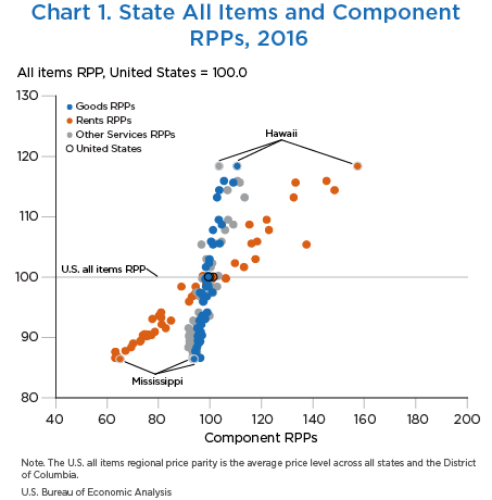
State all items RPPs for 2016 ranged from 118.4 for Hawaii to 86.4 for Mississippi (table 5). Hawaii’s price level is 18.4 percent higher than the national price level, and Mississippi’s price level is 13.6 percent lower. Price levels can also be directly compared across states by taking the ratio of the RPPs. Hawaii’s price level is 37.0 percent higher than Mississippi’s.
Among component RPPs, rents had the widest range (94.2 index points), from 63.2 in Alabama and West Virginia to 157.4 in Hawaii. Ranges were considerably narrower for goods RPPs (16.7 index points) and other services RPPs (21.9 index points). The wide range of rents RPPs across states is an important source of the variation in state all items RPPs (chart 1).
States with above average all items RPPs generally have rents RPPs that are higher than the other component RPPs. In addition, they generally have other services RPPs higher than goods RPPs. States like California, Connecticut, Maryland, New York, New Jersey, and the District of Columbia have higher average wages, consistent with having higher price levels for other services, compared with price levels for goods. Hawaii’s geographical isolation and added transportation and distribution costs led to a higher price level for goods, compared with the price level for other services.6
States with below average all items RPPs have rents RPPs that are lower than the other components. Additionally, these states’ other services RPPs are typically lower than their goods RPPs.
Table 5. State Real Per Capita Personal Income and Implicit Regional Price Deflator for 2015 and 2016 and Regional Price Parities for 2016
| Per capita personal income (dollars) | Real per capita personal income (chained (2009) dollars) | Implicit regional price deflator 1 | Regional price parities 2016 | ||||||||||
|---|---|---|---|---|---|---|---|---|---|---|---|---|---|
| 2015 | 2016 | Percent change | 2015 | 2016 | Percent change | 2015 | 2016 | Percent change | All items | Goods | Services | ||
| Rents | Other | ||||||||||||
| United States2 | 48,429 | 49,204 | 1.6 | 44,235 | 44,412 | 0.4 | 109.5 | 110.8 | 1.2 | 100.0 | 99.4 | 101.2 | 100.0 |
| Alabama | 38,238 | 38,918 | 1.8 | 40,356 | 40,689 | 0.8 | 94.7 | 95.6 | 1.0 | 86.6 | 96.2 | 63.2 | 93.3 |
| Alaska | 56,507 | 55,674 | −1.5 | 48,949 | 47,831 | −2.3 | 115.4 | 116.4 | 0.9 | 105.4 | 101.1 | 137.5 | 96.6 |
| Arizona | 39,731 | 40,546 | 2.1 | 37,889 | 38,265 | 1.0 | 104.9 | 106.0 | 1.0 | 95.9 | 97.4 | 91.8 | 97.2 |
| Arkansas | 39,060 | 39,722 | 1.7 | 40,967 | 41,371 | 1.0 | 95.3 | 96.0 | 0.7 | 86.9 | 94.7 | 63.8 | 93.3 |
| California | 54,664 | 56,308 | 3.0 | 44,022 | 44,562 | 1.2 | 124.2 | 126.4 | 1.8 | 114.4 | 103.6 | 148.4 | 106.8 |
| Colorado | 51,956 | 52,097 | 0.3 | 46,324 | 45,806 | −1.1 | 112.2 | 113.7 | 1.3 | 103.0 | 99.8 | 117.6 | 98.5 |
| Connecticut | 68,155 | 69,094 | 1.4 | 57,380 | 57,554 | 0.3 | 118.8 | 120.1 | 1.1 | 108.7 | 104.5 | 115.3 | 109.1 |
| Delaware | 47,069 | 47,837 | 1.6 | 43,036 | 43,223 | 0.4 | 109.4 | 110.7 | 1.2 | 100.2 | 99.1 | 97.1 | 103.2 |
| District of Columbia | 73,834 | 75,756 | 2.6 | 57,609 | 59,163 | 2.7 | 128.2 | 128.0 | −0.2 | 115.9 | 105.4 | 145.3 | 110.6 |
| Florida | 45,388 | 45,855 | 1.0 | 41,752 | 41,623 | −0.3 | 108.7 | 110.2 | 1.4 | 99.7 | 98.3 | 106.1 | 97.0 |
| Georgia | 41,020 | 42,146 | 2.7 | 40,545 | 41,407 | 2.1 | 101.2 | 101.8 | 0.6 | 92.1 | 96.7 | 81.2 | 94.7 |
| Hawaii | 48,823 | 50,358 | 3.1 | 37,583 | 38,514 | 2.5 | 129.9 | 130.8 | 0.7 | 118.4 | 110.5 | 157.4 | 103.5 |
| Idaho | 38,931 | 39,543 | 1.6 | 38,148 | 38,477 | 0.9 | 102.1 | 102.8 | 0.7 | 93.0 | 98.1 | 77.6 | 97.5 |
| Illinois | 50,745 | 51,679 | 1.8 | 46,796 | 47,302 | 1.1 | 108.4 | 109.3 | 0.8 | 98.9 | 98.9 | 98.4 | 99.2 |
| Indiana | 41,862 | 43,091 | 2.9 | 42,269 | 43,180 | 2.2 | 99.0 | 99.8 | 0.8 | 90.3 | 96.8 | 73.9 | 93.5 |
| Iowa | 45,800 | 46,056 | 0.6 | 46,372 | 46,230 | −0.3 | 98.8 | 99.6 | 0.8 | 90.2 | 95.2 | 75.1 | 91.8 |
| Kansas | 47,009 | 47,221 | 0.5 | 47,483 | 47,221 | −0.6 | 99.0 | 100.0 | 1.0 | 90.5 | 95.8 | 74.6 | 93.7 |
| Kentucky | 38,504 | 38,934 | 1.1 | 39,805 | 40,161 | 0.9 | 96.7 | 96.9 | 0.2 | 87.8 | 94.3 | 67.1 | 93.1 |
| Louisiana | 42,835 | 42,257 | −1.3 | 43,315 | 42,337 | −2.3 | 98.9 | 99.8 | 0.9 | 90.4 | 96.5 | 76.2 | 93.3 |
| Maine | 42,875 | 44,094 | 2.8 | 39,772 | 40,570 | 2.0 | 107.8 | 108.7 | 0.8 | 98.4 | 98.5 | 94.4 | 100.5 |
| Maryland | 56,197 | 57,972 | 3.2 | 46,879 | 47,936 | 2.3 | 119.9 | 120.9 | 0.8 | 109.5 | 103.4 | 122.0 | 107.0 |
| Massachusetts | 62,755 | 64,122 | 2.2 | 53,529 | 53,860 | 0.6 | 117.2 | 119.1 | 1.6 | 107.8 | 101.1 | 122.9 | 105.8 |
| Michigan | 43,072 | 44,231 | 2.7 | 42,252 | 42,931 | 1.6 | 101.9 | 103.0 | 1.1 | 93.3 | 97.3 | 81.0 | 96.3 |
| Minnesota | 51,139 | 51,990 | 1.7 | 48,049 | 48,283 | 0.5 | 106.4 | 107.7 | 1.2 | 97.5 | 100.9 | 95.4 | 94.9 |
| Mississippi | 34,804 | 35,524 | 2.1 | 37,007 | 37,222 | 0.6 | 94.0 | 95.4 | 1.5 | 86.4 | 93.8 | 65.0 | 93.3 |
| Missouri | 42,406 | 42,939 | 1.3 | 43,325 | 43,445 | 0.3 | 97.9 | 98.8 | 0.9 | 89.5 | 95.3 | 73.1 | 92.6 |
| Montana | 42,637 | 43,107 | 1.1 | 41,025 | 41,457 | 1.1 | 103.9 | 104.0 | 0.1 | 94.1 | 98.9 | 80.9 | 95.6 |
| Nebraska | 49,572 | 50,016 | 0.9 | 50,052 | 50,043 | 0.0 | 99.0 | 99.9 | 0.9 | 90.5 | 95.6 | 76.2 | 92.0 |
| Nevada | 43,128 | 43,579 | 1.0 | 40,461 | 40,510 | 0.1 | 106.6 | 107.6 | 0.9 | 97.4 | 96.1 | 94.7 | 101.1 |
| New Hampshire | 54,543 | 55,945 | 2.6 | 47,310 | 47,837 | 1.1 | 115.3 | 116.9 | 1.4 | 105.9 | 100.4 | 118.3 | 104.4 |
| New Jersey | 60,069 | 61,240 | 1.9 | 48,567 | 48,984 | 0.9 | 123.7 | 125.0 | 1.1 | 113.2 | 102.7 | 132.5 | 113.4 |
| New Mexico | 37,938 | 38,393 | 1.2 | 36,910 | 37,145 | 0.6 | 102.8 | 103.4 | 0.6 | 93.6 | 97.0 | 80.2 | 99.8 |
| New York | 58,324 | 59,289 | 1.7 | 46,281 | 46,416 | 0.3 | 126.0 | 127.7 | 1.3 | 115.6 | 109.0 | 133.2 | 111.6 |
| North Carolina | 41,351 | 42,203 | 2.1 | 41,546 | 42,020 | 1.1 | 99.5 | 100.4 | 0.9 | 90.9 | 96.3 | 78.6 | 93.3 |
| North Dakota | 55,643 | 54,801 | −1.5 | 55,110 | 54,213 | −1.6 | 101.0 | 101.1 | 0.1 | 91.5 | 95.0 | 82.8 | 91.6 |
| Ohio | 43,803 | 44,561 | 1.7 | 44,825 | 45,176 | 0.8 | 97.7 | 98.6 | 0.9 | 89.3 | 96.1 | 72.8 | 91.9 |
| Oklahoma | 43,999 | 42,717 | −2.9 | 44,879 | 43,458 | −3.2 | 98.0 | 98.3 | 0.3 | 89.0 | 95.5 | 70.1 | 93.3 |
| Oregon | 44,424 | 45,482 | 2.4 | 41,112 | 41,266 | 0.4 | 108.1 | 110.2 | 1.9 | 99.8 | 98.9 | 106.0 | 97.2 |
| Pennsylvania | 49,815 | 50,730 | 1.8 | 46,458 | 46,672 | 0.5 | 107.2 | 108.7 | 1.4 | 98.4 | 99.4 | 88.8 | 102.7 |
| Rhode Island | 49,744 | 50,373 | 1.3 | 45,768 | 45,795 | 0.1 | 108.7 | 110.0 | 1.2 | 99.6 | 98.3 | 100.6 | 100.3 |
| South Carolina | 38,802 | 39,527 | 1.9 | 39,362 | 39,613 | 0.6 | 98.6 | 99.8 | 1.2 | 90.3 | 96.7 | 77.1 | 93.3 |
| South Dakota | 47,882 | 48,051 | 0.4 | 49,620 | 49,243 | −0.8 | 96.5 | 97.6 | 1.1 | 88.3 | 94.9 | 69.3 | 91.5 |
| Tennessee | 42,156 | 43,338 | 2.8 | 42,980 | 43,496 | 1.2 | 98.1 | 99.6 | 1.5 | 90.2 | 96.2 | 75.8 | 93.3 |
| Texas | 46,787 | 46,204 | −1.2 | 44,211 | 43,148 | −2.4 | 105.8 | 107.1 | 1.2 | 96.9 | 97.2 | 93.7 | 98.6 |
| Utah | 39,775 | 41,018 | 3.1 | 37,657 | 38,142 | 1.3 | 105.6 | 107.5 | 1.8 | 97.3 | 96.7 | 94.3 | 100.3 |
| Vermont | 49,002 | 50,084 | 2.2 | 43,830 | 44,611 | 1.8 | 111.8 | 112.3 | 0.4 | 101.6 | 98.4 | 113.2 | 100.3 |
| Virginia | 52,189 | 52,941 | 1.4 | 46,544 | 46,856 | 0.7 | 112.1 | 113.0 | 0.8 | 102.3 | 99.6 | 109.7 | 100.8 |
| Washington | 53,119 | 54,632 | 2.8 | 46,304 | 46,863 | 1.2 | 114.7 | 116.6 | 1.7 | 105.5 | 103.7 | 116.1 | 101.9 |
| West Virginia | 36,566 | 36,673 | 0.3 | 37,734 | 37,906 | 0.5 | 96.9 | 96.7 | −0.2 | 87.6 | 94.4 | 63.2 | 94.9 |
| Wisconsin | 46,025 | 46,809 | 1.7 | 45,202 | 45,679 | 1.1 | 101.8 | 102.5 | 0.7 | 92.8 | 95.9 | 84.8 | 93.4 |
| Wyoming | 56,322 | 55,172 | −2.0 | 53,456 | 51,634 | −3.4 | 105.4 | 106.9 | 1.4 | 96.7 | 98.7 | 92.9 | 96.1 |
| Maximum | 73,834 | 75,756 | 3.2 | 57,609 | 59,163 | 2.7 | 129.9 | 130.8 | 1.9 | 118.4 | 110.5 | 157.4 | 113.4 |
| Minimum | 34,804 | 35,524 | −2.9 | 36,910 | 37,145 | −3.4 | 94.0 | 95.4 | −0.2 | 86.4 | 93.8 | 63.2 | 91.5 |
| Range | 39,030 | 40,232 | 6.1 | 20,699 | 22,018 | 6.1 | 35.9 | 35.4 | 2.1 | 32.0 | 16.7 | 94.2 | 21.9 |
- The implicit price deflator for the United States is equal to the national personal consumption expenditures price index, with a base of 2009.
- The U.S. all items regional price parity is the average price level across all states and the District of Columbia.
Note. Per capita personal income uses Census Bureau midyear population estimates available as of December 2017.
Metropolitan areas
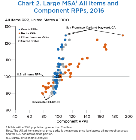
All items RPPs for large metropolitan areas—MSAs with a 2016 population greater than 2 million—ranged from 124.7 for San Francisco-Oakland-Hayward, CA, to 89.6 for Cincinnati, OH-KY-IN (table 6). San Francisco-Oakland-Hayward, CA’s price level is 24.7 percent higher than the national price level, and Cincinnati, OH-KY-IN’s is 10.4 percent lower. Taking the ratio of the RPPs, San Francisco-Oakland-Hayward, CA’s price level is 39.2 percent higher than Cincinnati, OH-KY-IN’s.
Among component RPPs for large MSAs, rents had the widest range (113.0 index points), from 77.9 in Cleveland-Elyria, OH, to 190.9 in San Francisco-Oakland-Hayward, CA. Across large MSAs, the ranges were considerably narrower for goods RPPs (16.4 index points) and other services RPPs (25.0 index points). Rents RPPs and other services RPPs had wider ranges for large MSAs, compared with states, suggesting that price levels vary more for more detailed geographies (tables 5 and 6).
As was seen with states, large MSAs with higher all items price levels generally have other services RPPs that are higher than the goods RPPs (chart 2). Large MSAs with lower-than-average price levels generally have other services RPPs that are lower than the goods RPPs.
Table 6. Large Metropolitan Areas Real Per Capita Personal Income and Implicit Regional Price Deflator for 2015 and 2016 and Regional Price Parities for 2016
| Per capita personal income (dollars) | Real per capita personal income (chained (2009) dollars) | Implicit regional price deflator 1 | Regional price parities 2016 | ||||||||||
|---|---|---|---|---|---|---|---|---|---|---|---|---|---|
| 2015 | 2016 | Percent change | 2015 | 2016 | Percent change | 2015 | 2016 | Percent change | All items | Goods | Services | ||
| Rents | Other | ||||||||||||
| United States2 | 48,451 | 49,246 | 1.6 | 44,255 | 44,450 | 0.4 | 109.5 | 110.8 | 1.2 | 100.0 | 99.0 | 101.7 | 100.1 |
| United States nonmetropolitan portion | 37,861 | 38,239 | 1.0 | 39,544 | 39,630 | 0.2 | 95.7 | 96.5 | 0.8 | 87.6 | 93.9 | 63.8 | 93.8 |
| Atlanta-Sandy Springs-Roswell, GA | 45,934 | 47,348 | 3.1 | 43,814 | 44,598 | 1.8 | 104.8 | 106.2 | 1.3 | 96.3 | 98.3 | 93.5 | 95.9 |
| Austin-Round Rock, TX | 51,128 | 51,566 | 0.9 | 47,171 | 46,820 | −0.7 | 108.4 | 110.1 | 1.6 | 100.0 | 97.9 | 117.2 | 93.4 |
| Baltimore-Columbia-Towson, MD | 55,468 | 57,189 | 3.1 | 47,360 | 48,393 | 2.2 | 117.1 | 118.2 | 0.9 | 107.2 | 102.8 | 116.0 | 105.2 |
| Boston-Cambridge-Newton, MA-NH | 68,712 | 70,157 | 2.1 | 57,067 | 57,317 | 0.4 | 120.4 | 122.4 | 1.7 | 111.1 | 101.4 | 141.0 | 107.2 |
| Charlotte-Concord-Gastonia, NC-SC | 45,609 | 46,679 | 2.3 | 44,798 | 45,297 | 1.1 | 101.8 | 103.0 | 1.2 | 93.5 | 97.4 | 86.5 | 93.4 |
| Chicago-Naperville-Elgin, IL-IN-WI | 54,518 | 55,621 | 2.0 | 48,177 | 48,625 | 0.9 | 113.2 | 114.4 | 1.1 | 103.8 | 100.1 | 114.8 | 102.2 |
| Cincinnati, OH-KY-IN | 47,787 | 48,668 | 1.8 | 48,836 | 49,278 | 0.9 | 97.9 | 98.8 | 0.9 | 89.6 | 94.6 | 78.7 | 90.9 |
| Cleveland-Elyria, OH | 48,019 | 48,968 | 2.0 | 48,829 | 49,292 | 0.9 | 98.3 | 99.3 | 1.0 | 90.2 | 95.9 | 77.9 | 90.9 |
| Columbus, OH | 46,904 | 47,725 | 1.8 | 46,335 | 46,550 | 0.5 | 101.2 | 102.5 | 1.3 | 93.0 | 96.9 | 84.2 | 93.4 |
| Dallas-Fort Worth-Arlington, TX | 51,062 | 51,099 | 0.1 | 46,868 | 46,270 | −1.3 | 108.9 | 110.4 | 1.4 | 100.2 | 99.0 | 103.2 | 99.9 |
| Denver-Aurora-Lakewood, CO | 57,081 | 56,892 | −0.3 | 49,837 | 48,728 | −2.2 | 114.5 | 116.8 | 2.0 | 106.0 | 100.8 | 127.9 | 99.3 |
| Detroit-Warren-Dearborn, MI | 47,310 | 48,692 | 2.9 | 45,119 | 46,061 | 2.1 | 104.9 | 105.7 | 0.8 | 95.9 | 98.2 | 86.7 | 99.3 |
| Houston-The Woodlands-Sugar Land, TX | 53,859 | 51,913 | −3.6 | 48,845 | 46,378 | −5.1 | 110.3 | 111.9 | 1.5 | 101.6 | 96.2 | 103.2 | 107.3 |
| Indianapolis-Carmel-Anderson, IN | 48,207 | 49,681 | 3.1 | 47,673 | 48,602 | 1.9 | 101.1 | 102.2 | 1.1 | 92.8 | 97.2 | 83.0 | 93.5 |
| Kansas City, MO-KS | 48,394 | 48,514 | 0.2 | 47,250 | 47,011 | −0.5 | 102.4 | 103.2 | 0.8 | 93.7 | 96.5 | 82.4 | 97.1 |
| Las Vegas-Henderson-Paradise, NV | 41,915 | 42,284 | 0.9 | 39,216 | 39,247 | 0.1 | 106.9 | 107.7 | 0.7 | 97.8 | 95.4 | 96.5 | 102.0 |
| Los Angeles-Long Beach-Anaheim, CA | 55,585 | 57,160 | 2.8 | 43,409 | 44,087 | 1.6 | 128.0 | 129.7 | 1.3 | 117.7 | 104.8 | 165.4 | 107.4 |
| Miami-Fort Lauderdale-West Palm Beach, FL | 51,454 | 52,210 | 1.5 | 44,034 | 44,037 | 0.0 | 116.9 | 118.6 | 1.5 | 107.6 | 100.6 | 129.4 | 100.9 |
| Minneapolis-St. Paul-Bloomington, MN-WI | 55,599 | 56,723 | 2.0 | 49,894 | 50,311 | 0.8 | 111.4 | 112.7 | 1.2 | 102.3 | 103.9 | 110.1 | 96.7 |
| New York-Newark-Jersey City, NY-NJ-PA | 64,679 | 65,846 | 1.8 | 48,846 | 48,992 | 0.3 | 132.4 | 134.4 | 1.5 | 122.0 | 109.9 | 154.9 | 115.9 |
| Orlando-Kissimmee-Sanford, FL | 39,337 | 40,169 | 2.1 | 36,907 | 37,210 | 0.8 | 106.6 | 108.0 | 1.3 | 98.0 | 97.9 | 104.8 | 93.4 |
| Philadelphia-Camden-Wilmington, PA-NJ-DE-MD | 57,327 | 58,589 | 2.2 | 49,654 | 50,209 | 1.1 | 115.5 | 116.7 | 1.0 | 105.9 | 101.2 | 111.3 | 107.9 |
| Phoenix-Mesa-Scottsdale, AZ | 41,443 | 42,218 | 1.9 | 39,235 | 39,455 | 0.6 | 105.6 | 107.0 | 1.3 | 97.1 | 97.2 | 97.7 | 96.5 |
| Pittsburgh, PA | 50,622 | 51,187 | 1.1 | 49,296 | 49,264 | −0.1 | 102.7 | 103.9 | 1.2 | 94.3 | 98.1 | 78.9 | 98.1 |
| Portland-Vancouver-Hillsboro, OR-WA | 49,217 | 50,489 | 2.6 | 44,660 | 45,034 | 0.8 | 110.2 | 112.1 | 1.7 | 101.7 | 99.0 | 117.7 | 97.5 |
| Riverside-San Bernardino-Ontario, CA | 35,762 | 36,807 | 2.9 | 30,619 | 31,088 | 1.5 | 116.8 | 118.4 | 1.4 | 107.4 | 101.6 | 117.6 | 106.8 |
| Sacramento--Roseville--Arden-Arcade, CA | 50,026 | 51,370 | 2.7 | 45,079 | 45,693 | 1.4 | 111.0 | 112.4 | 1.3 | 102.0 | 95.4 | 117.6 | 102.0 |
| St. Louis, MO-IL | 48,876 | 49,519 | 1.3 | 49,347 | 49,480 | 0.3 | 99.0 | 100.1 | 1.1 | 90.8 | 94.3 | 82.7 | 91.4 |
| San Antonio-New Braunfels, TX | 44,127 | 44,284 | 0.4 | 42,912 | 42,595 | −0.7 | 102.8 | 104.0 | 1.2 | 94.4 | 97.5 | 90.2 | 93.4 |
| San Diego-Carlsbad, CA | 53,963 | 55,168 | 2.2 | 42,663 | 43,063 | 0.9 | 126.5 | 128.1 | 1.3 | 116.3 | 100.1 | 167.6 | 105.6 |
| San Francisco-Oakland-Hayward, CA | 81,241 | 84,675 | 4.2 | 60,324 | 61,639 | 2.2 | 134.7 | 137.4 | 2.0 | 124.7 | 110.7 | 190.9 | 111.0 |
| Seattle-Tacoma-Bellevue, WA | 62,883 | 64,553 | 2.7 | 52,574 | 53,003 | 0.8 | 119.6 | 121.8 | 1.8 | 110.5 | 106.3 | 134.0 | 104.0 |
| Tampa-St. Petersburg-Clearwater, FL | 43,352 | 43,807 | 1.0 | 39,917 | 39,843 | −0.2 | 108.6 | 109.9 | 1.2 | 99.8 | 96.5 | 103.5 | 101.8 |
| Washington-Arlington-Alexandria, DC-VA-MD-WV | 65,155 | 66,733 | 2.4 | 50,150 | 50,861 | 1.4 | 129.9 | 131.2 | 1.0 | 119.1 | 105.4 | 166.4 | 110.7 |
| Maximum | 81,241 | 84,675 | 4.2 | 60,324 | 61,639 | 2.2 | 134.7 | 137.4 | 2.0 | 124.7 | 110.7 | 190.9 | 115.9 |
| Minimum | 35,762 | 36,807 | −3.6 | 30,619 | 31,088 | −5.1 | 97.9 | 98.8 | 0.7 | 89.6 | 94.3 | 77.9 | 90.9 |
| Range | 45,479 | 47,868 | 7.8 | 29,705 | 30,551 | 7.3 | 36.8 | 38.6 | 1.3 | 35.1 | 16.4 | 113.0 | 25.0 |
- The implicit price deflator for the United States is equal to the national personal consumption expenditures price index, with a base of 2009.
- The U.S. all items regional price parity is the average price level across all metropolitan areas and the U.S. nonmetropolitan portion.
Note. Per capita personal income uses Census Bureau midyear population estimates available as of March 2017.
Per capita personal income
Per capita personal income (PCPI) is nominal personal income divided by population. Estimating real PCPI for states and MSAs requires two price adjustments. The first adjustment estimates PCPI at RPPs by controlling for relative price differences across regions. The second adjustment uses the national personal consumption expenditures (PCE) price index to control for price changes over time. The product of a region’s RPP and the PCE price index for a given year is the region’s implicit regional price deflator (IRPD). Change in the IRPD is an implicit measure of regional inflation. For a more detailed example of how real PCPI is estimated, see the box “Using Regional Price Parities (RPPs) to Estimate Real Personal Income.”
States
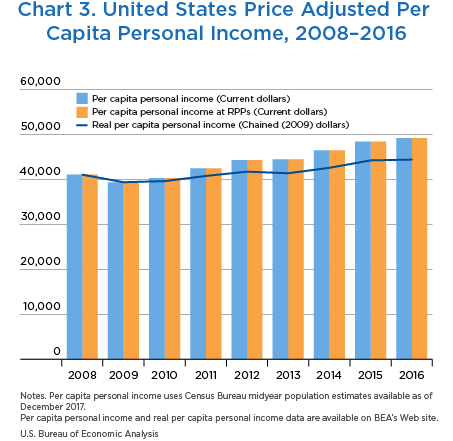
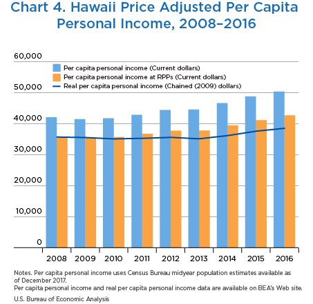
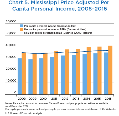
Charts 3, 4, and 5 show the impact of the two adjustments for the United States, Hawaii, and Mississippi for 2008 to 2016, respectively. The United States shows no difference between the PCPI and PCPI at RPPs, because the U.S. all items RPP—the average across all states and components—is 100.0 for all years. Hawaii’s 2016 PCPI at RPPs ($42,669) is lower than its PCPI ($50,358) because it has an RPP greater than 100.0 (table 7). Above average price levels yield a downward adjustment. By contrast, Mississippi’s 2016 PCPI at RPPs ($41,238) is higher than its PCPI ($35,524). Mississippi’s lower price level yields an upward adjustment. The application of the RPPs narrows the range of incomes across states from $40,232 for PCPI to $24,394 for PCPI at RPPs.
The difference between PCPI at RPPs and real PCPI for any state reflects the adjustment using the PCE price index. Charts 3 through 5 show no difference between the PCPI at RPPs and real PCPI in the base year 2009, because the PCE price index is 100.0. Hawaii’s 2016 PCPI is higher than its real PCPI ($38,514). Mississippi’s 2016 PCPI is lower than its real PCPI ($37,222). These relationships hold for every year from 2008 to 2016, reflecting each state’s relative price levels and national price levels over time. Adjusting state PCPI at RPPs with the PCE price index narrows the range to $22,018 for real PCPI.
| Per capita personal income (current dollars) |
Per capita personal income at RPPs (current dollars) |
Real per capita personal income (chained (2009) dollars) |
|
|---|---|---|---|
| United States | 49,204 | 49,204 | 44,412 |
| Hawaii | 50,358 | 42,669 | 38,514 |
| Mississippi | 35,524 | 41,238 | 37,222 |
| Across all states | |||
| Maximum | 75,756 | 65,547 | 59,163 |
| Minimum | 35,524 | 41,153 | 37,145 |
| Range | 40,232 | 24,394 | 22,018 |
Notes. Real personal income data for all states are available on BEA’s website.
Per capita personal income uses Census Bureau midyear population estimates available as of December 2017.
Large metropolitan areas
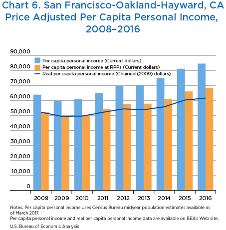
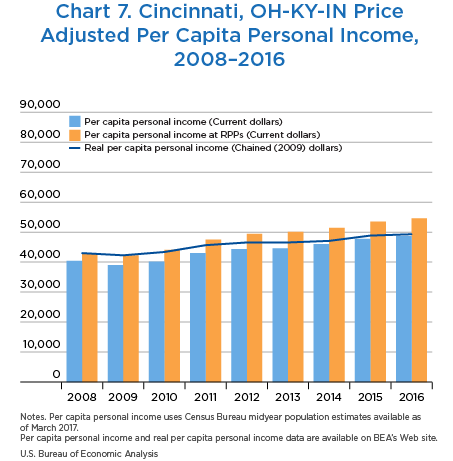
The adjustment process for the San Francisco-Oakland-Hayward CA, and for Cincinnati, OH-KY-IN, for 2008 to 2016 are shown in charts 6 and 7, respectively. San Francisco-Oakland-Hayward, CA’s 2016 PCPI at RPP ($68,289) is lower than its PCPI ($84,675) because it has an RPP above 100.0 (table 8). Cincinnati, OH-KY-IN’s 2016 PCPI at RPPs ($54,595) is higher than its PCPI ($48,668); its lower price level yields an upward adjustment. Across large MSAs, the application of the RPPs narrows the range from $47,868 for PCPI to $33,847 for PCPI at RPPs.
The difference between PCPI at RPPs and real PCPI for any MSA reflects the adjustment using the PCE price index. San Francisco-Oakland-Hayward, CA’s 2016 PCPI is higher than its real PCPI ($61,639). Cincinnati, OH-KY-IN’s 2016 PCPI is lower than its real PCPI ($49,278). As with the state examples above, these relationships hold for every year from 2008 to 2016, reflecting their lower relative prices and national price levels over time. The application of the PCE price index narrows the range of incomes to $30,551 for real PCPI.
| Per capita personal income (current dollars) |
Per capita personal income at RPPs (current dollars) |
Real per capita personal income (chained (2009) dollars) |
|
|---|---|---|---|
| United States | 49,246 | 49,246 | 44,450 |
| United States nonmetropolitan portion | 38,239 | 43,906 | 39,630 |
| San Francisco-Oakland-Hayward, CA | 84,675 | 68,289 | 61,639 |
| Cincinnati, OH-KY-IN | 48,668 | 54,595 | 49,278 |
| Across large metropolitan areas | |||
| Maximum | 84,675 | 68,289 | 61,639 |
| Minimum | 36,807 | 34,442 | 31,088 |
| Range | 47,868 | 33,847 | 30,551 |
Notes. Real personal income data for all metropolitan areas are available on BEA’s website.
Per capita personal income uses Census Bureau midyear population estimates available as of March 2017.
On March 6, 2018, the Bureau of Economic Analysis (BEA) released Arts and Cultural Production Satellite Account (ACPSA) data for 2015; it also released updated data for 2013 and 2014. With the most recent data release, BEA, for the first time, included state-level statistics for value added by arts and cultural industries for 2001 to 2015.
Value added is defined as the gross output of an industry or sector less its intermediate inputs. It measures the contribution of an industry or a sector to gross domestic product (GDP). Its usefulness lies in its ability to provide a broad measure of value created by a specific sector within the economy.
Nationally, ACPSA value added increased 6.3 percent in 2015 to $763.6 billion dollars (table 9). ACPSA value added can be split into two categories: (1) core arts and cultural production industries and (2) supporting arts and cultural production industries. The core industries increased 8.1 percent in 2015 to $153.0 billion dollars. The core industries consist of industries whose output is identified as primarily contributing to arts and culture. The supporting industries increased 5.9 percent in 2015 to $583.8 billion dollars. Supporting industries consist of industries whose output supports the core category through publication, dissemination of the creative process, or other supportive functions.
| Industry | 2014 | 2015 | Dollar change | Percent change |
|---|---|---|---|---|
| Total | 718,555 | 763,569 | 45,014 | 6.3 |
| Core arts and cultural production | 141,558 | 152,954 | 11,396 | 8.1 |
| Performing arts | 48,278 | 52,942 | 4,664 | 9.7 |
| Performing arts companies | 16,627 | 17,801 | 1,174 | 7.1 |
| Promoters of performing arts and similar events | 9,045 | 10,453 | 1,408 | 15.6 |
| Agents/managers for artists | 2,496 | 2,706 | 210 | 8.4 |
| Independent artists, writers, and performers | 20,110 | 21,982 | 1,872 | 9.3 |
| Museums | 5,176 | 5,261 | 85 | 1.6 |
| Design services | 79,783 | 86,109 | 6,326 | 7.9 |
| Advertising | 31,198 | 33,099 | 1,901 | 6.1 |
| Architectural services | 15,288 | 17,168 | 1,880 | 12.3 |
| Landscape architectural services | 2,650 | 2,779 | 129 | 4.9 |
| Interior design services | 8,019 | 8,875 | 856 | 10.7 |
| Industrial design services | 1,707 | 1,791 | 84 | 4.9 |
| Graphic design services | 7,473 | 8,073 | 600 | 8.0 |
| Computer systems design | 3,132 | 3,430 | 298 | 9.5 |
| Photography and photofinishing services | 9,630 | 10,150 | 520 | 5.4 |
| All other design services | 687 | 743 | 56 | 8.2 |
| Fine arts education | 3,270 | 3,422 | 152 | 4.6 |
| Education services | 5,050 | 5,219 | 169 | 3.3 |
| Supporting arts and cultural production | 551,007 | 583,765 | 32,758 | 5.9 |
| Art support services | 107,149 | 110,652 | 3,503 | 3.3 |
| Information services | 341,331 | 363,051 | 21,720 | 6.4 |
| Publishing | 75,331 | 77,694 | 2,363 | 3.1 |
| Motion pictures | 93,091 | 99,280 | 6,189 | 6.6 |
| Sound recording | 13,398 | 14,854 | 1,456 | 10.9 |
| Broadcasting | 122,368 | 127,844 | 5,476 | 4.5 |
| Other information services | 37,144 | 43,379 | 6,235 | 16.8 |
| Manufacturing | 14,430 | 15,039 | 609 | 4.2 |
| Construction | 9,409 | 10,195 | 786 | 8.4 |
| Wholesale and transportation industries | 30,775 | 33,517 | 2,742 | 8.9 |
| Retail industries | 47,912 | 51,311 | 3,399 | 7.1 |
| All other industries | 25,991 | 26,851 | 860 | 3.3 |
Within the core arts, the performing arts and design services industries were the leading contributors to growth. Performing arts, which increased $4.76 billion dollars (9.7 percent) in 2015, includes performing arts companies, promoters of performing arts and similar events, and independent artists, writers, and performers. Performing arts companies increased $1.2 billion dollars (7.1 percent); promoters of performing arts and similar events increased $1.4 billion dollars (15.6 percent); while independent artists, writers, and performers increased $1.9 billion dollars (9.3 percent). Design services, which increased $6.3 billion dollars (7.9 percent) in 2015, was paced by increases in advertising and architectural services. The increase in supporting arts industries was led by increases in other information services and motion pictures, where both industries increased $6.2 billion dollars (16.8 percent and 6.6 percent, respectively) in 2015.
Performing arts
In terms of value added, California, New York, Florida, and Tennessee accounted for 63.6 percent of the national total for performing arts (table 10). Among the four states, Tennessee was the outlier as its economy was smaller than the other three. In terms of overall GDP in 2015, California, New York, and Florida were also among top four largest states while Tennessee ranked 18th.
| Millions of dollars | Percent of U.S. performing arts companies total | |
|---|---|---|
| United States | 52,942 | 100.0 |
| California | 18,131 | 34.2 |
| New York | 10,217 | 19.3 |
| Florida | 2,749 | 5.2 |
| Tennessee | 2,557 | 4.8 |
| Texas | 1,879 | 3.5 |
| Nevada | 1,387 | 2.6 |
| Illinois | 1,188 | 2.2 |
| Ohio | 1,086 | 2.1 |
| Massachusetts | 1,084 | 2.0 |
| New Jersey | 1,025 | 1.9 |
Tennessee has played a critical role in the development of many forms of American popular music, including rock and roll, blues, country, and rockabilly. Beale Street in Memphis is considered by many to be the birthplace of the blues. Memphis is also home to Sun Records, where musicians such as Elvis Presley, Johnny Cash, Carl Perkins, Jerry Lee Lewis, Roy Orbison, and Charlie Rich began their recording careers and where rock and roll took shape in the 1950s. With Memphis being the birthplace of rock ’n roll and Nashville nicknamed “Music City” because it is considered the center of the country music recording industry, Tennessee’s performing arts industry is driven by its outsized role in the music industry.
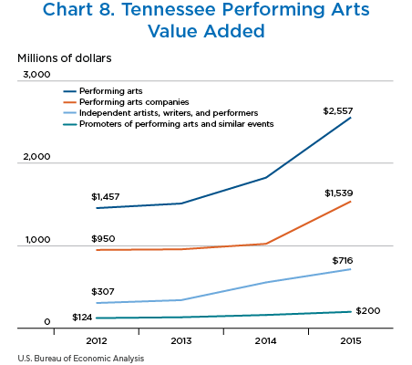
The performing arts industry in Tennessee has seen large increases in value added, employment, and average compensation since 2012. Between 2012 and 2015, value added in Tennessee grew 75.5 percent from $1.5 billion to $2.6 billion dollars (chart 8). Within performing arts, from 2012 to 2015, value added for performing arts companies increased $589 million dollars (62.0 percent). Valued added for independent artists, writers, and performers grew $409 million dollars (133.2 percent) from 2012 to 2015.
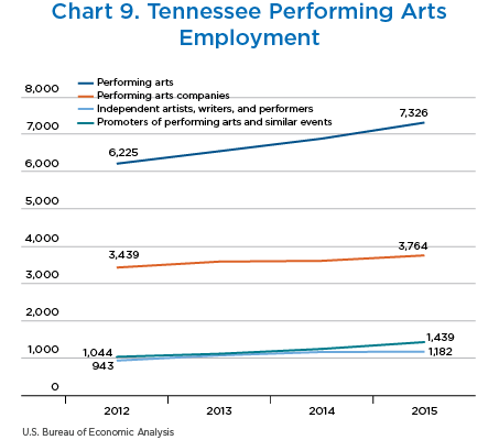
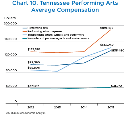
Employment (the number of jobs) and the average compensation for those jobs in the performing arts industry have also experienced double-digit increases between 2012 and 2015. Employment increased from 6,225 to 7,326 (17.7 percent), while average compensation in those performing arts jobs increased from $99,390 to $135,480 (36.3 percent) (chart 9 and chart 10). The increase in employment was led by increases in employment in promoters of performing arts and similar events and performing arts companies with 37.8 percent and 9.5 percent growth, respectively, from 2012 to 2015. The increase in average compensation was led by significant increases in compensation in performing arts companies and independent artists, writers, and performers. From 2012 to 2015, average compensation in performing arts companies increased from $132,578 to $189,097. Average compensation for independent artists, writers, and performers increased from $85,806 to $143,049.
Motion pictures
Unsurprisingly, California and New York account for 77.8 percent of the national total of value added for the motion pictures industry in 2015 (table 11). In 2015, motion pictures contributed $49.1 billion dollars to California’s economy, representing 2.0 percent of California’s total GDP. In New York, motion pictures contributed $28.2 billion dollars to the state economy, representing 1.9 percent of its economy. Louisiana, whose overall GDP is the 24th largest among states, had the third-largest share of value added in the motion pictures industry at $2.7 billion dollars (1.1 percent of its economy).
| Millions of dollars | Percent of U.S. motion picture total | |
|---|---|---|
| United States | 99,280 | 100.0 |
| California | 49,120 | 49.5 |
| New York | 28,150 | 28.4 |
| Louisiana | 2,699 | 2.7 |
| Texas | 2,122 | 2.1 |
| Florida | 1,624 | 1.6 |
| Connecticut | 1,583 | 1.6 |
| Georgia | 1,463 | 1.5 |
| New Jersey | 1,349 | 1.4 |
| Tennessee | 1,220 | 1.2 |
| Pennsylvania | 969 | 1.0 |
Several factors contribute to the development of motion pictures and film within a specific location. These factors include natural resources—such as the weather, landscape, and local scenery—as well as access to capital, such as the existing labor force (human capital) and production-related infrastructure (physical capital)—all of which impact the cost of production. New York was the center of early film production due to access to skilled labor and existing infrastructure. The growth in popularity of motion pictures contributed to the demand that necessitated year-round production, and California weather was uniquely suited to provide year-round production.
While advancements in digital effects have decreased the reliance of film production on a specific physical locale, the cost of production spending continues to be important in motion picture development. One way that states or localities have tried to attract motion picture production has been by providing financial incentives to mitigate the cost of production. These incentives include grants, rebates, or tax credits, with various additional requirements, such as minimum spender caps. The rationale for offering these incentives is not only to entice out-of-state production companies to film in-state and increase in-state spending but also to allow for the long-term development of the motion pictures industry, related infrastructure, and skilled labor within the state. Louisiana has actively provided financial incentives for the motion picture industry beginning in 2002. That year, the Louisiana state legislature established (1) an incremental 10 percent tax credit on both production spending and resident payroll for projects totaling $300,000–$1 million and (2) a 15 percent production spending tax credit and a 20 percent resident payroll tax credit for projects over $1 million.7
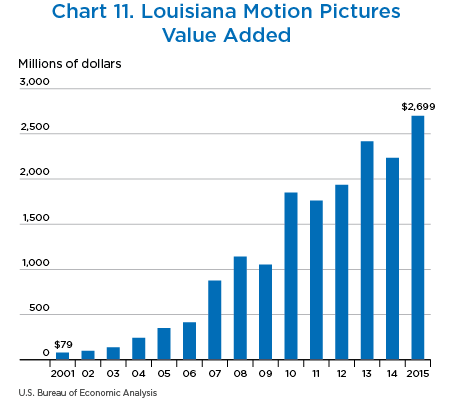
Since 2001, valued added in the motion pictures industry in Louisiana has increased significantly, and the industry has become a bigger part of the state’s economy. In 2001, the motion pictures industry contributed $79 million dollars to Louisiana’s economy, representing less than 0.1 percent of Louisiana’s total GDP (chart 11). From 2001 to 2015, valued added in the motion pictures industry has grown over 3,000 percent with jumps in growth in 2007, 2010, 2013, and 2015. In 2015, the motion pictures industry contributed 1.1 percent to the Louisiana economy.
- Real GDP in Louisiana’s petroleum and coal products manufacturing fell 23 percent in 2017.
- BEA estimates of wages and salaries by state and industry, rather than earnings, were used for mining and real estate. U.S. Department of Agriculture estimates of farm income and expenses by state were used to estimate agriculture GDP.
- In addition, new state and local government finance data for fiscal year 2015 for property taxes and severance taxes (among other things) from the Census Bureau were incorporated.
- The Office of Management and Budget defines MSAs as one or more counties with a high degree of social and economic integration, with a core urban population of 50,000 or more.
- RPPs are calculated for the 50 states and the District of Columbia, state metropolitan and nonmetropolitan portions, and metropolitan areas. Estimates for metropolitan areas include an estimate for the nonmetropolitan portion of the United States to provide complete coverage of all U.S. counties.
- See Bettina H. Aten, “Regional Price Parities and Real Regional Income for the United States,”
Social Indicators Research 131.1 (2017): 123–143. - Office of Entertainment Industry Development, Louisiana Department of Economic Development, Inc. (2003). The Economic Impact Analysis of Louisiana’s Entertainment Tax Credit Programs. Baton Rouge, LA: Loren C. Scott & Associates.

