
New County-Level Gross Domestic Product
On December 12, 2018, the Bureau of Economic Analysis (BEA) released prototype measures of gross domestic product (GDP) by county. GDP by county is a measure of the market value of final goods and services produced within a county area in a particular period. While other measures of county economies rely mainly on labor market data, these statistics are the first of their kind to incorporate multiple data sources that capture trends in labor, revenue, and value of production. As a result, the capital-intensive industries are captured more fully than when measured solely by labor data. These statistics represent another step forward in meeting BEA's long-standing goal of providing a more detailed and accurate geographic distribution of the nation's economic activity.
GDP by county statistics provide a richer picture not only of the distribution of national economic output but also of national economic trends and their manifestation at finer and alternative levels of geographic detail. They can be used to inform resource allocation decisions and support economic development strategies that target areas with the greatest need by identifying strengths and weaknesses of local economies. GDP by county statistics can also support research into understanding local economic dynamics, the longer-term impacts of different development strategies, and the effectiveness of incentive programs used to support these strategies.
Potential uses of the statistics
BEA statistics on GDP by county can be used to meet a variety of research, business, and policy needs. The statistics can also help answer important questions related to the size and condition of local area economies, industrial composition, and comparative growth trends.
General assessments. The statistics provide a tool to quickly gain a broad understanding of an overall economy. The data provide an overview of growth and size in absolute and relative terms. Some important questions these data can answer are as follows:
- What is the size of a county's economy?
- Is a county's economy growing or declining?
- What industries are driving a county's economic growth?
- How does the growth in one county’s economy compare with growth in other counties, in the state, or in the nation?
- What has been the trend in economic growth over time in a county's economy?
Economic research. GDP by county statistics facilitate research projects by providing large quantities of data in the form of a cross-sectional time series. These projects require high-quality data that are consistently defined. Some research topics these data can facilitate are as follows:
- Indepth analysis of the distribution of national economic output
- National economic trends and their manifestation at finer and alternative levels of geographic detail
- Local economic dynamics
- Longer-term impacts of different development strategies
- Economic development strategies that target areas with the greatest need by identifying strengths and weaknesses of local economies
- Effectiveness of incentive programs used to support these strategies
Business and policy decisions. GDP by county statistics provide information that helps assess the relative performance of geographic areas in terms of size and growth. The statistics also indicate where industries are concentrated. These are important factors for many business or policy decisions. The following are some of the decisions the data can inform:
- Business owners and policymakers can decide how to allocate resources based on strengths and weaknesses of their economy.
- Policymakers can recognize the systematic variation in the value of economies of small counties that are not large enough to be part of metropolitan areas but have large enough economies to have a meaningful impact on their state's and the nation’s economy.
- Local officials and regional planners concerned with addressing the developmental needs of their areas can identify the strengths and weaknesses of their economy and make informed decisions. Additionally, they can evaluate the long-term impacts of different economic policies in their region.
- County governments can assess the future economic growth potential of their counties and evaluate how different industries and government sectors are changing.
- County governments can use the statistics to prepare promotional materials to attract investors.
- Manufacturers interested in relocating to a local county can distinguish whether goods-producing or services-providing industries are performing better in that county.
These prototype estimates were prepared by BEA in response to demand for more indepth economic data about counties. In conjunction with their release, BEA is requesting feedback and comments on these prototype statistics to assist in improving their quality, reliability, and usefulness.
The data sources and methods discussed in this section are the culmination of over a decade of planning, development, and refinement. Following the 2007 release of GDP by metropolitan area—an area defined as a combination of one or more counties—efforts to release a more local area measure began.1 While the GDP by metropolitan area series effectively measured metropolitan area economic activity and identified trends in industries and locales, an even more thorough and local measure was needed. This was particularly important for counties in which composition of growth differed from their metropolitan area counterparts and for more rural counties outside metropolitan areas.
Data sources
The most significant improvement in the GDP by county statistics, when compared with the previous county measures that form the basis of GDP by metropolitan area, is more robust source data. The new prototype statistics incorporate additional source data, which more fully capture the returns to the capital factor of production. These include source data from the Economic Census, BEA local area personal income, and the National Establishment Time Series (NETS) Database, all of which are used for many industries. Where available or when required, additional data are incorporated to measure economic activity. Table A compares the data sources used for the GDP by metropolitan area statistics with those used for the prototype GDP by county statistics. The table also lists the data sources used to corroborate the statistics.
| Input source data | ||
|---|---|---|
| Metropolitan area methodology | Prototype county methodology | |
| Earnings | Earnings | |
| GDP by state | GDP by state | |
| Compensation | ||
| Proprietors’ income | ||
| Economic Census | ||
| QCEW wages | ||
| NETS Database | ||
| FDIC deposits by bank branch | ||
| EIA net electricity generation | ||
| USDA Census of Agriculture sales and payroll | ||
| Corroborative source data | ||
| Metropolitan area methodology | Prototype county methodology | |
| LexisNexis | LexisNexis | |
| WARN reports | WARN reports | |
| FEMA disaster data | FEMA disaster data | |
| USDA crop insurance data | USDA crop insurance data | |
| IncentivesMonitor | ||
| State Business Incentives Database | ||
| State Economic Development Program Expenditures Database | ||
| Conway Analytics | ||
| DrillingEdge | ||
- EIA
- Energy Information Agency
- FDIC
- Federal Deposit Insurance Corporation
- FEMA
- Federal Emergency Management Agency
- GDP
- Gross domestic product
- NETS
- National Establishment Times Series
- QCEW
- Quarterly Census of Employment and Wages
- USDA
- United States Department of Agriculture
- WARN
- Worker Adjustment and Retraining Notification
The Economic Census is conducted every 5 years and captures data from roughly four million U.S. companies.2 It contains data from companies across the economic spectrum (large and small and goods-producing and services-producing) and is a critical source for many BEA statistical products. The GDP by county statistics rely heavily on this data. Value-added and payroll data are used in the estimation of manufacturing industries, while receipts and payroll data are used in the estimation of services-producing industries.
GDP by county statistics incorporate BEA local area personal income statistics.3 Earnings, which is compensation of employees (wages and salaries and supplements to wages) plus proprietors’ income, is used in most of the methodologies as one of the input variables. For select industries, wages, instead of compensation, are used as the primary source data, as shown in Appendix A.
The Bureau of Labor Statistics Quarterly Census of Employment and Wages (QCEW) publishes a quarterly count of employment and wages by industry reported by employers. This report covers more than 97 percent of U.S. jobs and is available at the county, metropolitan area, state, and national levels.4 These wage data supplement the Economic Census data when a value is either not available or is suppressed.
NETS is a time series database consisting of annual data from Dun & Bradstreet for over 59 million establishments from 1990–2015. This collection of data includes a wealth of information on establishments and microestablishments, such as location, ownership structure, industrial operation structure, years of operation, relocation, industry classification, births and deaths, sales, and employment. The prototype statistics use annual sales data from NETS to supplant Economic Census data when a value either is not available or is suppressed.
The following data sources are specific to one industry:
- The U.S. Department of Agriculture conducts a Census of Agriculture every 5 years, capturing sales and payroll data by county from the farming community.
- The Federal Deposit Insurance Corporation (FDIC) Summary of Deposits publishes bank deposits by branch in each county for every active bank.
- The Energy Information Agency (EIA) produces data on net electricity generation by megawatt hours for all counties.
Corroborative information
BEA evaluated the quality of the prototype statistics using a variety of independent data sources from trade associations, company publications, and subscription databases. The sources were selected to identify an area’s largest employers, to characterize the local business climate, and to reveal market and labor trends in selected industries.
Data on economic development incentives and incentivized deals provide critical information on new and expanded business. The State Business Incentives Database is a searchable database of incentive programs used by states for strategic business attraction. The database includes 2,110 incentive programs enacted across the country, organized according to program category, program type, geographic focus, and business need.
The State Economic Development Program Expenditures Database is a compilation of data on state investments in economic development that categorizes expenses. The database enables cross-state and time series comparisons in various economic development expense categories including business attraction, technology transfer, workforce preparation and development, and business financing.
IncentivesMonitor is a database that tracks, collects, and analyzes information on domestic and foreign corporate investment projects that have received state incentives. The data details new investments, expansion investments, and relocation- or restructuring-related investments associated with the corresponding state incentive program. To date, 55,500 deals have been tracked, totaling $206 billion in value, $2 trillion in capital investment, and 8 million jobs, and representing 42,400 unique companies.
The Conway Analytics database contains more than 315,000 new plant and expansion records going back to 1989. It reports on new construction and office and industrial leases that create 20 or more new jobs, cover 20,000 square feet or more, and have at least $1 million in total investment. Database entries include project location, company name, product manufactured or services performed, North American Industry Classification System (NAICS) code, facility type, and stage of development.
DrillingEdge provides energy production data used to corroborate the geographic assignment and relative production level of local areas for the oil and gas industry. Oil production is reported in barrels, while gas production is reported in thousands of cubic feet.
BEA identified several sources of information on local labor trends. LexisNexis and state departments of labor publish data on the largest employers and their employment levels, which can be used to analyze industry trends for local economies. In addition, Worker Adjustment and Retraining Notification (WARN) reports, also from state governments, show which industries experienced a decline in their workforce.
The farms industry is one of the most challenging industries to measure, partly due to the effect weather has on the industry. The U.S. Department of Agriculture publishes data on crop losses by county. Information from the Federal Emergency Management Agency on the timeline of severe weather events and the magnitude of losses indicates which counties are affected and the relative impact.
Collectively, these sources are used to analyze and refine the statistics. Additional sources may be included in future analysis.
The calculation of GDP by county statistics starts with the creation of current-dollar statistics for each industry within a county. The “Methods” section below begins with the methodology for goods-producing and services-producing industries, followed by the methodology for intercensal years.
Methods
Estimation of county values often involves the distribution of a state value to the counties based on the county value of an indicator data series. An indicator series is a data set with a known distribution. In the context of GDP by county estimation, the indicator series is assumed to be similar to the unknown county distribution of the state total. The prototype methodology applies the indicator in one of three ways for most industries: economic census years, extrapolation, or interpolation. Appendix A lists the methodology used for each industry. While we publish at a higher level of industry detail, the statistics are generally computed at the three-digit NAICS (2012) level to maximize the probative value of source data. As discussed in the “Next Steps” section, future work includes exploration on how the published level of industry detail can be expanded.
Economic census years
The Census Bureau publishes the Economic Census every 5 years. The procedure used to distribute a state total according to an indicator series in economic census years is commonly referred to as “allocation” because a state control total is “allocated” or “shared out” to the counties. Similarly, it can be said that an allocation procedure reconciles a first estimate to a control total. In general, GDP by county statistics are derived by applying an indicator series to GDP by state to compute GDP by county; this is done for each detailed industry listed in Appendix A. In this prototype, earnings data are augmented by Economic Census value added, payroll, and/or receipts data, combining both a capital and labor component to form a more comprehensive indicator. Production measurement in capital-intensive industries is better informed by the addition of value added or receipts—measures of returns to capital. The degree to which unsuppressed Economic Census data are available informs the methodology. When Economic Census data are not available, NETS sales data and QCEW wages are used to estimate the suppressed values. The methodology for Economic Census years can be further distinguished for goods- and services-producing industries.
(Private) goods-producing industries. Goods-producing industries use Economic Census value added in conjunction with BEA compensation of employees and proprietors’ income to distribute GDP by state to counties. The three data sources are combined to create a weighted indicator series (see the box “Weight Formulas Applied in the Computation of County GDP”).
Data from the Census Bureau is adjusted to account for differences in industry coverage and classification between the Census Bureau and BEA. The Census Bureau value-added data are multiplied by the ratio of BEA wages and salaries to Census Bureau payrolls by county and by industry. This adjustment is done on the assumption that the ratio would be 1.0 if there were no differences in coverage and classification of establishments between the two data series. Due to the nature of the data and to maintain confidentiality, some county and industry values in the value-added series are suppressed. Where these suppressions occur, NETS sales and QCEW wages data are used to fill in the suppressed Economic Census data to maintain the time series. After adjusting Census Bureau value-added data, the sum-of-county-adjusted value added for the goods-producing industries are reconciled with the state industry accounts value added, yielding estimates of GDP by county and by industry.
(Private) services-producing industries. Economic Census receipts, compensation of employees, and proprietors’ income data are used to distribute GDP by state to counties. The three data sources are combined to create a weighted indicator series (see the box “Weight Formulas Applied in the Computation of County GDP”). The methodology differs from the goods-producing methodology in that receipts data are used because value-added data are not available for services-producing industries. Based on the availability of Economic Census receipts data, the weights for the components of earnings increase as the extent of Economic Census suppressions increase.
Extrapolation
We use extrapolation for the industries that use Economic Census data and Census of Agriculture data, which are available every 5 years. An extrapolation technique using NETS sales data (S) computes GDP by county for the years following the most recent Economic Census when the next Economic Census data are not yet available. To extrapolate, one would need to decide what value to assign to the extrapolator (Δ)—the vehicle which applies a percent change to a base series to create the extrapolated value. Ideally, a series with a similar growth pattern is used to extrapolate. Assigning Δ a value of 1.0 keeps the ratio between GDP by county and S constant during the extrapolation period (Δ is 1.0 plus the annual growth rate, so a value of 1.0 implies a zero-growth rate for the ratio.) However, it may be possible, through regression analysis or other means, to identify a time trend in the relationship between GDP by county and S. The value may then be non-zero, but the algebra of the extrapolation would be the same.
Interpolation
We use interpolation for the industries that use Economic Census data and Census of Agriculture data, which are available every 5 years. All data interpolations used in the GDP by county estimates are growth rate interpolations. That is, they are geometric rather than linear interpolations. Geometric interpolation is applied using NETS sales data during the intercensal years.
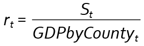
The NETS sales data, S, are available for all years in the time series; therefore, the interpolated values for GDP by county can be tied to the available values of S by interpolating the ratio between the two series. In the years for which values of GDP by county are available, compute the ratios between the values of GDP by county and the values of the related series S:
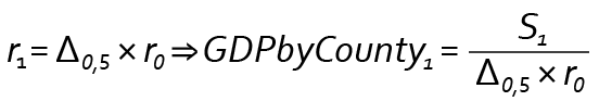
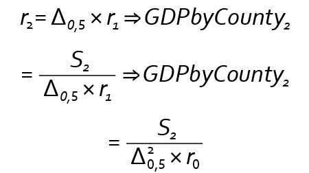
The interpolated values of these ratios are then computed by applying the average annual growth rate between available ratio values, which are directly computable just every 5 years in the current example:
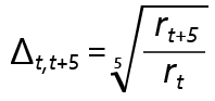
The value is the annual geometric factor (1.0 plus the average annual growth rate in the ratio) for computing interpolated values of the ratios between the related data series S and the missing values (GDP by county) and so on until all the missing values of GDP by county have been computed.
Other methodologies
QCEW wages are used to distribute GDP by state to counties where the Economic Census data do not reflect the production in an industry. This can be due to the nature of the industry or limited coverage by the Economic Census data or receipts that are not a reliable indicator of industry production compared against its inputs.
The farms, banking, and utilities industries each have separate indicator series specific to their industry. In Census years, the farms industry relies on sales data from the USDA Census of Agriculture to distribute GDP by state to the county level. For the banking industry, the distribution of GDP by state to counties is based on the county share of bank branch deposits. FDIC Summary of Deposits data are used to compute the shares of bank branch deposits for each county, which in turn, are used to distribute GDP by state. Deposit levels have proven to be an accurate indication of the location of GDP produced by this industry and a reasonable indication of trends in the industry’s growth. The utilities industry’s distribution of GDP by state to counties is based on the county share of net electricity generation from EIA. Electricity generation provides a reasonable indication of trends in the industry’s growth.
For a few industries, such as mining and construction, a return to capital component series is not available, and the county share of earnings data are used to distribute GDP by state to counties. Earnings are considered a reasonable indicator of relative levels of economic activity. Many of these industries are part of the methodology refinements discussed in the “Next Steps” section.
Chained-dollar statistics
Real GDP by county was prepared in chained (2012) dollars. Real GDP by county is an inflation-adjusted measure of each county based on national prices. These measures are important when making comparisons over time and when calculating growth.
The real statistics for each industry in each county are derived by applying national chain-type price indexes from the BEA Industry Economic Accounts to the statistics on current-dollar GDP by county for the detailed industries.5 For aggregate industry sectors and total GDP, real GDP by county statistics are derived using the same chain-type index formula that is used in the national accounts.
To the extent that a county’s output is produced and sold in national markets at relatively uniform prices (or sold locally at national prices), real GDP by county should accurately capture the relative differences in the mix of goods and services that metropolitan areas produce. However, these statistics do not capture county-to-county differences in the prices that may exist locally for some goods and services.6
The prototype GDP by county statistics highlight the diversity of the nation’s local economies. Not only do counties vary in size, they vary by industry composition and growth. This section will explore these factors and how trends differed for metropolitan and nonmetropolitan counties.
Highlights 2012–2015
- Overall, 1,931 of 3,113 counties grew in 2015.
- Private services-producing industries was the leading contributor in most counties.
- Growth in metropolitan counties outpaced growth in nonmetropolitan counties.
- The U.S. economy has been in transition from goods-producing industries to services-producing industries.
- In 2015, seven counties produced more than half of their state GDP.
Comparison of methods
The prototype methodology to compute GDP by county was compared with the former earnings-based approach used to compute GDP by metropolitan area. Both sets of county statistics were aggregated to metropolitan areas.7 The difference was measured as the mean absolute percent difference (MAPD).
MAPDs were analyzed according to the largest industry group in each metropolitan area. Table B shows the number of metropolitan areas predominated by each industry and the associated MAPD. The overall MAPD for all 383 metropolitan areas was 4.6 percent.
In 361 metropolitan areas, services-producing industries comprise the largest share of GDP. These metropolitan areas have a MAPD of 4.3 percent, suggesting the earnings-based approach did a good job, while indicating additional source data was still beneficial.
In 10 metropolitan areas, goods-producing industries comprise the largest share of GDP. As expected, these metropolitan areas have the largest MAPD (13.6 percent). The additional source data had the most impact on these industries, particularly due to their capital-intensive nature.
| Leading industry | Number of metropolitan areas | MAPD of total gross domestic product (percent) |
|---|---|---|
| Goods-producing industries | 10 | 13.6 |
| Services-producing industries | 361 | 4.3 |
| Government | 12 | 3.4 |
| Total | 383 | 4.6 |
Table C breaks down the results by size of metropolitan area and industry—small metropolitan areas have populations under 500,000; medium metropolitan areas have a population between 500,000 and 2 million; and large metropolitan areas have populations over 2 million. The total MAPD for the three groups ranges from 5.3 percent to 1.4 percent and is the smallest for large metropolitan areas. As expected, goods-producing industries had the largest differences; differences were largest in small metropolitan areas. In addition, small metropolitan areas had the largest difference for both goods- and services-producing industries. The prototype methodology had the most impact on goods-producing industries, as illustrated in the goods-producing column. Overall, 270 out of 383 metropolitan areas have MAPDs less than 5 percent; 352 have MAPDs less than 10 percent; and 366 have MAPDs less than 15 percent.
| Size of metropolitan area | Total GDP | Goods-producing industries | Services-producing industries | Government |
|---|---|---|---|---|
| Large | 1.4 | 4.0 | 2.0 | 0.0 |
| Medium | 3.5 | 5.7 | 4.4 | 0.0 |
| Small | 5.3 | 10.5 | 6.5 | 0.0 |
GDP by size
The largest 15 counties produced nearly 25 percent of the nation’s GDP. Five of these counties are located in California; the rest are in eight other states. By contrast, only 10 percent of the nation’s GDP is produced by the smallest 2,381 counties. Within the context of their states, counties have shares of their respective state, ranging from 78.2 percent (Honolulu County, HI) to 0.0003 percent (Loving County, TX). The distribution of GDP by county is shown in chart 1.

[Click chart to expand]
Importance of counties to states
According to data from the World Bank, the two largest counties in 2015, Los Angeles County, CA ($691.9 billion) and New York County, NY ($690.0 billion), would rank as the world›s 18th and 19th largest national economies, respectively.8 GDP in 25 counties was greater than $100 billion—greater than the GDP of Ecuador—the 61st largest national economy in 2015. GDP in 301 counties was greater than $10 billion—greater than the GDP of Madagascar—the 138th largest national economy in 2015. And GDP in 1,420 counties was greater than $1 billion—greater than the GDP of Grenada—the 186th largest national economy in 2015.
In 2015, there were seven states (excluding the District of Columbia) in which a single county produced more than half of their state GDP: Honolulu County, HI (78.2 percent); Clark County, NV (72.6 percent); Maricopa County, AZ (72.5 percent), New Castle County, DE (69.6 percent); Providence County, RI (60.4 percent); King County, WA (55.9 percent); and Salt Lake County, UT (53.3 percent). Additionally, excluding New Castle County, DE, these counties contributed more than half to their state’s total GDP growth in 2015.
Transition from goods to services
The U.S. economy has been in transition from goods-producing industries to services-producing industries across the entire BEA historic GDP by industry timeline, dating back to 1947. Services-producing industries are the largest industry category for the nation, all states, and the District of Columbia, as well as 361 of 383 metropolitan areas. The county data show further evidence in this continuing shift. Between 2012 and 2015, 3.1 percent of the nation’s counties’ leading industries changed from goods-producing industries or government to services-producing industries (charts 2 and 3). The numbers show the shift from goods- to services-producing industries is more pronounced in nonmetropolitan counties. From 2012 to 2015, the number of counties with services-producing industries as the largest industry increased by 1 percent in metropolitan counties, from 1,003 to 1,014, and 4.3 percent in nonmetropolitan counties, from 1,245 to 1,329 (table C). As of 2015, services-producing industries was the largest industry in all counties in the New England region. The largest shift to services-producing industries occurred in the Plains region, where 61 of the 490 nonmetropolitan counties (12.4 percent) transitioned from goods-producing as their largest industry to services-producing.

[Click chart to expand]

[Click chart to expand]
Overall, services-producing industries are the largest industry group for both metropolitan and nonmetropolitan counties. However, services-producing industries comprise a larger share of metropolitan counties than nonmetropolitan counties (table D). Furthermore, industry composition varies significantly among counties. In 2015, services-producing industries ranged from 5.3 percent in Menominee County, WI, to 94.5 percent in Butte County, ID. Goods-producing industries ranged from 0.3 percent in Menominee County, WI, to 92.0 percent in Sullivan County, MO. Government ranged from 1.5 percent in Broomfield County, CO, to 94.4 percent in Menominee County, WI. Butte County, ID, and Broomfield County, CO, are metropolitan counties, while the other counties listed above are all nonmetropolitan counties. These are just some of the indications of diversity that can influence economic trends among the nation’s counties.
| County type | Total counties | Industry | 2012 | 2015 | Difference | |||
|---|---|---|---|---|---|---|---|---|
| Count | Percent | Count | Percent | Count | Percent | |||
| Metropolitan | 1,149 | Goods | 118 | 10.3 | 111 | 9.7 | −7 | -0.6 |
| Services | 1,003 | 87.3 | 1,014 | 88.3 | 11 | 1.0 | ||
| Government | 28 | 2.4 | 24 | 2.1 | −4 | -0.3 | ||
| Nonmetropolitan | 1,964 | Goods | 643 | 32.7 | 563 | 28.7 | −80 | -4.1 |
| Services | 1,245 | 63.4 | 1,329 | 67.7 | 84 | 4.3 | ||
| Government | 76 | 3.9 | 72 | 3.7 | −4 | -0.2 | ||
Given the experimental nature of the GDP by county estimates, BEA is interested in the views of its data users on the prototype methodologies and the appropriate level of industry detail. BEA is especially interested in the following:
- Do some prototype estimates overstate or understate economic activity, based on specialized knowledge of the local area economy?
- Do users prefer less detailed estimates by industry with fewer suppressions or more detailed industry estimates with the necessary suppressions?
Subject to data users’ evaluation and comments, BEA plans to monitor revisions to these estimates; conduct research to improve methodologies for the construction, mining, real estate, and transportation industries; and evaluate methods to accelerate the timeline of these estimates. BEA plans to release estimates for 2001–2018 on December 12, 2019. BEA will also analyze suppression patterns and determine the level of industry detail for official release.
Please e-mail your comments to BEA at gdpbycounty@bea.gov.
| Industry name | NAICS (2012) code | Methodology used | Weight formula |
|---|---|---|---|
| Farms | 111–112 | Farms | n.a. |
| Forestry, fishing, and related activities | 113–115 | Wages | n.a. |
| Oil and gas extraction | 211 | Earnings | n.a. |
| Mining (except oil and gas) | 212 | Earnings | n.a. |
| Support activities for mining | 213 | Earnings | n.a. |
| Utilities | 22 | Utilities | n.a. |
| Construction | 23 | Earnings | n.a. |
| Wood product manufacturing | 321 | Goods-producing methodology | 1 |
| Nonmetallic mineral product manufacturing | 327 | Goods-producing methodology | 1 |
| Primary metal manufacturing | 331 | Goods-producing methodology | 1 |
| Fabricated metal product manufacturing | 332 | Goods-producing methodology | 1 |
| Machinery manufacturing | 333 | Goods-producing methodology | 1 |
| Computer and electronic product manufacturing | 334 | Goods-producing methodology | 1 |
| Electrical equipment, appliance, and component manufacturing | 335 | Goods-producing methodology | 1 |
| Motor vehicles, bodies and trailers, and parts manufacturing | 3361–3363 | Goods-producing methodology | 1 |
| Other transportation equipment manufacturing | 3364–3366, 3369 | Goods-producing methodology | 1 |
| Furniture and related product manufacturing | 337 | Goods-producing methodology | 1 |
| Miscellaneous manufacturing | 339 | Goods-producing methodology | 1 |
| Food and beverage and tobacco products manufacturing | 311–312 | Goods-producing methodology | 1 |
| Textile mills and textile product mills manufacturing | 313–314 | Goods-producing methodology | 1 |
| Apparel, leather, and allied products manufacturing | 315–316 | Goods-producing methodology | 1 |
| Paper manufacturing | 322 | Goods-producing methodology | 1 |
| Printing and related support activities manufacturing | 323 | Goods-producing methodology | 1 |
| Petroleum and coal products manufacturing | 324 | Goods-producing methodology | 1 |
| Chemical manufacturing | 325 | Goods-producing methodology | 1 |
| Plastics and rubber products manufacturing | 326 | Goods-producing methodology | 1 |
| Wholesale trade | 42 | Services-producing methodology | 3 |
| Retail trade | 44–45 | Services-producing methodology | 3 |
| Air transportation | 481 | Earnings | n.a. |
| Rail transportation | 482 | Earnings | n.a. |
| Water transportation | 483 | Services-producing methodology | 2 |
| Truck transportation | 484 | Services-producing methodology | 2 |
| Transit and ground passenger transportation | 485 | Services-producing methodology | 2 |
| Pipeline transportation | 486 | Services-producing methodology | 2 |
| Other transportation and support activities | 487–488, 492 | Services-producing methodology | 2 |
| Warehousing and storage | 493 | Services-producing methodology | 2 |
| Publishing industries (except internet) | 511 | Services-producing methodology | 2 |
| Motion picture and sound recording industries | 512 | Wages | n.a. |
| Broadcasting (except internet) and telecommunications | 515, 517 | Services-producing methodology | 2 |
| Data processing, hosting, and other information services | 518, 519 | Services-producing methodology | 2 |
| Monetary Authorities - Central bank, credit intermediation, and related services | 521–522 | Banking | n.a. |
| Securities, commodity contracts, and other financial investments and related activities | 523 | Services-producing methodology | 2 |
| Insurance carriers and related activities | 524 | Services-producing methodology | 2 |
| Funds, trusts, and other financial vehicles | 525 | Services-producing methodology | 2 |
| Real estate | 531 | Earnings | n.a. |
| Rental and leasing services and lessors of nonfinancial intangible assets | 532–533 | Services-producing methodology | 3 |
| Legal services | 5411 | Services-producing methodology | 3 |
| Computer systems design and related services | 5415 | Services-producing methodology | 3 |
| Miscellaneous professional, scientific, and technical services | 5412–5414, 5416–5419 | Services-producing methodology | 3 |
| Management of companies and enterprises | 55 | Wages | n.a. |
| Administrative and support services | 561 | Services-producing methodology | 3 |
| Waste management and remediation services | 562 | Services-producing methodology | 3 |
| Educational services | 61 | Services-producing methodology | 3 |
| Hospitals | 622 | Services-producing methodology | 3 |
| Nursing and residential care facilities | 623 | Services-producing methodology | 3 |
| Ambulatory health care services | 621 | Services-producing methodology | 3 |
| Social assistance | 624 | Services-producing methodology | 3 |
| Performing arts, spectator sports, museums, and related activities | 711–712 | Services-producing methodology | 3 |
| Amusement, gambling, and recreation industries | 713 | Services-producing methodology | 3 |
| Accommodation | 721 | Services-producing methodology | 3 |
| Food services and drinking places | 722 | Services-producing methodology | 3 |
| Other services (except government and government enterprises) | 81 | Services-producing methodology | 3 |
| Federal civilian | n.a. | Earnings | n.a. |
| Military | n.a. | Wages | n.a. |
| State and local | n.a. | Earnings | n.a. |
- n.a.
- Not available
- NAICS
- North American Industry Classification System
| Real GDP | Percent change from preceding period | ||||||||
|---|---|---|---|---|---|---|---|---|---|
| Thousands of chained (2012) dollars | Rank in state | Percent change | Rank in state | ||||||
| 2012 | 2013 | 2014 | 2015 | 2015 | 2013 | 2014 | 2015 | 2015 | |
| Autauga | 1,383,941 | 1,322,416 | 1,312,668 | 1,412,939 | 24 | −4.4 | −0.7 | 7.6 | 7 |
| Baldwin | 5,599,194 | 6,218,819 | 6,247,887 | 5,981,958 | 7 | 11.1 | 0.5 | −4.3 | 57 |
| Barbour | 639,833 | 687,532 | 663,462 | 708,778 | 36 | 7.5 | −3.5 | 6.8 | 8 |
| Bibb | 297,560 | 314,380 | 305,472 | 291,780 | 56 | 5.7 | −2.8 | −4.5 | 59 |
| Blount | 632,761 | 683,949 | 661,352 | 778,131 | 33 | 8.1 | −3.3 | 17.7 | 2 |
| Bullock | 191,052 | 185,250 | 170,520 | 169,621 | 65 | −3.0 | −8.0 | −0.5 | 43 |
| Butler | 514,216 | 510,470 | 488,051 | 510,960 | 43 | −0.7 | −4.4 | 4.7 | 12 |
| Calhoun | 4,073,476 | 3,918,440 | 3,780,726 | 3,750,456 | 11 | −3.8 | −3.5 | −0.8 | 45 |
| Chambers | 567,650 | 613,470 | 653,977 | 667,159 | 40 | 8.1 | 6.6 | 2.0 | 18 |
| Cherokee | 443,582 | 467,206 | 435,311 | 412,342 | 48 | 5.3 | −6.8 | −5.3 | 60 |
| Chilton | 715,347 | 764,758 | 737,867 | 739,287 | 34 | 6.9 | −3.5 | 0.2 | 36 |
| Choctaw | 524,082 | 488,313 | 501,011 | 470,631 | 46 | −6.8 | 2.6 | −6.1 | 62 |
| Clarke | 700,361 | 708,413 | 710,848 | 717,501 | 35 | 1.1 | 0.3 | 0.9 | 28 |
| Clay | 232,085 | 261,017 | 261,037 | 265,276 | 58 | 12.5 | 0.0 | 1.6 | 23 |
| Cleburne | 249,914 | 248,261 | 254,896 | 284,071 | 57 | −0.7 | 2.7 | 11.4 | 3 |
| Coffee | 1,084,201 | 1,088,751 | 1,112,386 | 1,237,578 | 28 | 0.4 | 2.2 | 11.3 | 4 |
| Colbert | 2,393,641 | 2,640,273 | 2,757,890 | 2,876,934 | 13 | 10.3 | 4.5 | 4.3 | 14 |
| Conecuh | 256,668 | 258,811 | 248,926 | 246,082 | 61 | 0.8 | −3.8 | −1.1 | 48 |
| Coosa | 118,371 | 123,568 | 128,630 | 125,727 | 67 | 4.4 | 4.1 | −2.3 | 53 |
| Covington | 978,150 | 1,022,605 | 997,884 | 999,820 | 31 | 4.5 | −2.4 | 0.2 | 35 |
| Crenshaw | 387,037 | 418,156 | 375,890 | 382,326 | 50 | 8.0 | −10.1 | 1.7 | 20 |
| Cullman | 2,301,223 | 2,364,721 | 2,314,983 | 2,299,075 | 18 | 2.8 | −2.1 | −0.7 | 44 |
| Dale | 2,756,921 | 2,819,437 | 2,689,058 | 2,676,064 | 16 | 2.3 | −4.6 | −0.5 | 40 |
| Dallas | 1,125,070 | 1,112,684 | 1,090,446 | 1,042,780 | 30 | −1.1 | −2.0 | −4.4 | 58 |
| DeKalb | 1,485,948 | 1,688,899 | 1,656,070 | 1,684,337 | 20 | 13.7 | −1.9 | 1.7 | 21 |
| Elmore | 1,396,129 | 1,497,274 | 1,511,276 | 1,537,004 | 23 | 7.2 | 0.9 | 1.7 | 22 |
| Escambia | 1,056,880 | 1,038,718 | 1,015,770 | 996,597 | 32 | −1.7 | −2.2 | −1.9 | 50 |
| Etowah | 2,607,155 | 2,580,422 | 2,529,908 | 2,537,130 | 17 | −1.0 | −2.0 | 0.3 | 33 |
| Fayette | 260,930 | 264,086 | 261,565 | 262,842 | 59 | 1.2 | −1.0 | 0.5 | 31 |
| Franklin | 720,181 | 780,664 | 705,590 | 702,000 | 37 | 8.4 | −9.6 | −0.5 | 41 |
| Geneva | 406,627 | 430,780 | 418,366 | 437,309 | 47 | 5.9 | −2.9 | 4.5 | 13 |
| Greene | 246,604 | 230,026 | 223,915 | 198,632 | 64 | −6.7 | −2.7 | −11.3 | 65 |
| Hale | 226,473 | 264,111 | 242,492 | 251,413 | 60 | 16.6 | −8.2 | 3.7 | 15 |
| Henry | 259,333 | 290,103 | 297,272 | 294,677 | 55 | 11.9 | 2.5 | −0.9 | 46 |
| Houston | 4,122,576 | 4,164,957 | 4,104,867 | 4,030,351 | 10 | 1.0 | −1.4 | −1.8 | 49 |
| Jackson | 1,327,414 | 1,371,337 | 1,352,030 | 1,254,897 | 27 | 3.3 | −1.4 | −7.2 | 64 |
| Jefferson | 42,005,734 | 41,051,828 | 40,026,017 | 40,267,211 | 1 | −2.3 | −2.5 | 0.6 | 30 |
| Lamar | 276,202 | 265,718 | 255,999 | 245,499 | 62 | −3.8 | −3.7 | −4.1 | 56 |
| Lauderdale | 2,325,961 | 2,402,292 | 2,350,008 | 2,298,453 | 19 | 3.3 | −2.2 | −2.2 | 52 |
| Lawrence | 728,868 | 679,450 | 587,433 | 477,055 | 45 | −6.8 | −13.5 | −18.8 | 67 |
| Lee | 4,668,575 | 5,206,210 | 5,405,859 | 5,980,010 | 8 | 11.5 | 3.8 | 10.6 | 5 |
| Limestone | 2,704,953 | 2,862,219 | 2,988,146 | 3,150,965 | 12 | 5.8 | 4.4 | 5.4 | 10 |
| Lowndes | 357,630 | 383,814 | 361,485 | 337,731 | 53 | 7.3 | −5.8 | −6.6 | 63 |
| Macon | 437,454 | 438,399 | 399,303 | 387,698 | 49 | 0.2 | −8.9 | −2.9 | 55 |
| Madison | 20,870,718 | 20,963,910 | 21,209,589 | 21,398,559 | 2 | 0.4 | 1.2 | 0.9 | 29 |
| Marengo | 574,835 | 587,910 | 598,854 | 592,137 | 42 | 2.3 | 1.9 | −1.1 | 47 |
| Marion | 694,213 | 738,945 | 685,390 | 683,158 | 39 | 6.4 | −7.2 | −0.3 | 39 |
| Marshall | 2,576,840 | 2,782,135 | 2,649,827 | 2,686,505 | 14 | 8.0 | −4.8 | 1.4 | 25 |
| Mobile | 17,983,867 | 17,594,349 | 17,259,624 | 17,221,153 | 3 | −2.2 | −1.9 | −0.2 | 38 |
| Monroe | 623,195 | 550,283 | 583,397 | 688,517 | 38 | −11.7 | 6.0 | 18.0 | 1 |
| Montgomery | 13,104,289 | 13,143,702 | 13,142,737 | 13,439,829 | 4 | 0.3 | 0.0 | 2.3 | 17 |
| Morgan | 4,183,977 | 4,275,717 | 4,300,763 | 4,312,042 | 9 | 2.2 | 0.6 | 0.3 | 34 |
| Perry | 179,161 | 176,489 | 169,305 | 165,089 | 66 | −1.5 | −4.1 | −2.5 | 54 |
| Pickens | 274,572 | 329,564 | 336,787 | 346,536 | 51 | 20.0 | 2.2 | 2.9 | 16 |
| Pike | 1,142,083 | 1,132,379 | 1,206,137 | 1,278,942 | 26 | −0.8 | 6.5 | 6.0 | 9 |
| Randolph | 335,720 | 367,563 | 339,375 | 340,952 | 52 | 9.5 | −7.7 | 0.5 | 32 |
| Russell | 1,201,079 | 1,187,457 | 1,327,831 | 1,395,915 | 25 | −1.1 | 11.8 | 5.1 | 11 |
| St. Clair | 1,458,587 | 1,571,339 | 1,568,338 | 1,585,838 | 21 | 7.7 | −0.2 | 1.1 | 27 |
| Shelby | 8,391,914 | 8,565,897 | 8,885,097 | 9,735,187 | 5 | 2.1 | 3.7 | 9.6 | 6 |
| Sumter | 240,325 | 243,873 | 246,068 | 231,168 | 63 | 1.5 | 0.9 | −6.1 | 61 |
| Talladega | 2,422,265 | 2,732,987 | 2,699,773 | 2,685,765 | 15 | 12.8 | −1.2 | −0.5 | 42 |
| Tallapoosa | 1,004,256 | 981,983 | 1,034,275 | 1,048,934 | 29 | −2.2 | 5.3 | 1.4 | 24 |
| Tuscaloosa | 10,199,891 | 9,989,993 | 9,330,105 | 9,323,664 | 6 | −2.1 | −6.6 | −0.1 | 37 |
| Walker | 1,577,706 | 1,599,522 | 1,599,977 | 1,565,304 | 22 | 1.4 | 0.0 | −2.2 | 51 |
| Washington | 690,145 | 697,845 | 744,718 | 637,320 | 41 | 1.1 | 6.7 | −14.4 | 66 |
| Wilcox | 296,863 | 298,271 | 314,351 | 318,680 | 54 | 0.5 | 5.4 | 1.4 | 26 |
| Winston | 484,525 | 512,695 | 481,939 | 490,932 | 44 | 5.8 | −6.0 | 1.9 | 19 |
| Real GDP | Percent change from preceding period | ||||||||
|---|---|---|---|---|---|---|---|---|---|
| Thousands of chained (2012) dollars | Rank in state | Percent change | Rank in state | ||||||
| 2012 | 2013 | 2014 | 2015 | 2015 | 2013 | 2014 | 2015 | 2015 | |
| Aleutians East Borough | 111,032 | 133,530 | 133,387 | 164,319 | 21 | 20.3 | −0.1 | 23.2 | 2 |
| Aleutians West Census Area | 363,807 | 399,436 | 378,922 | 386,878 | 15 | 9.8 | −5.1 | 2.1 | 11 |
| Anchorage Municipality | 27,571,441 | 26,135,685 | 25,071,285 | 25,548,523 | 1 | −5.2 | −4.1 | 1.9 | 12 |
| Bethel Census Area | 699,678 | 674,796 | 656,391 | 640,556 | 10 | −3.6 | −2.7 | −2.4 | 19 |
| Bristol Bay Borough | 104,109 | 115,158 | 109,022 | 104,246 | 23 | 10.6 | −5.3 | −4.4 | 24 |
| Denali Borough | 254,910 | 232,016 | 234,118 | 217,615 | 19 | −9.0 | 0.9 | −7.0 | 26 |
| Dillingham Census Area | 224,497 | 237,621 | 244,880 | 236,493 | 17 | 5.8 | 3.1 | −3.4 | 22 |
| Fairbanks North Star Borough | 5,489,188 | 5,467,710 | 5,649,698 | 5,675,709 | 3 | −0.4 | 3.3 | 0.5 | 14 |
| Haines Borough | 64,685 | 71,862 | 71,322 | 69,321 | 28 | 11.1 | −0.8 | −2.8 | 20 |
| Hoonah-Angoon Census Area | 54,407 | 60,500 | 59,461 | 69,987 | 27 | 11.2 | −1.7 | 17.7 | 3 |
| Juneau City and Borough | 2,279,424 | 2,266,269 | 2,293,619 | 2,220,596 | 6 | −0.6 | 1.2 | −3.2 | 21 |
| Kenai Peninsula Borough | 3,140,724 | 3,375,189 | 3,316,261 | 3,317,994 | 4 | 7.5 | −1.7 | 0.1 | 15 |
| Ketchikan Gateway Borough | 802,339 | 747,975 | 751,924 | 758,517 | 9 | −6.8 | 0.5 | 0.9 | 13 |
| Kodiak Island Borough | 741,748 | 780,404 | 808,878 | 827,596 | 8 | 5.2 | 3.6 | 2.3 | 10 |
| Kusilvak Census Area | 127,397 | 123,478 | 128,853 | 122,856 | 22 | −3.1 | 4.4 | −4.7 | 25 |
| Lake and Peninsula Borough | 68,147 | 70,349 | 71,291 | 73,772 | 26 | 3.2 | 1.3 | 3.5 | 8 |
| Matanuska-Susitna Borough | 2,233,060 | 2,209,831 | 2,284,002 | 2,356,921 | 5 | −1.0 | 3.4 | 3.2 | 9 |
| Nome Census Area | 402,931 | 395,458 | 405,640 | 389,845 | 14 | −1.9 | 2.6 | −3.9 | 23 |
| North Slope Borough | 8,920,976 | 7,251,453 | 6,596,616 | 6,516,645 | 2 | −18.7 | −9.0 | −1.2 | 17 |
| Northwest Arctic Borough | 628,118 | 667,707 | 659,604 | 594,456 | 11 | 6.3 | −1.2 | −9.9 | 27 |
| Petersburg Borough | 146,199 | 131,078 | 134,911 | 171,559 | 20 | −10.3 | 2.9 | 27.2 | 1 |
| Prince of Wales-Hyder Census Area | 229,136 | 247,470 | 243,495 | 252,879 | 16 | 8.0 | −1.6 | 3.9 | 7 |
| Sitka City and Borough | 404,873 | 415,731 | 429,511 | 428,095 | 13 | 2.7 | 3.3 | −0.3 | 16 |
| Skagway Municipality | 67,100 | 76,612 | 69,115 | 74,486 | 25 | 14.2 | −9.8 | 7.8 | 5 |
| Southeast Fairbanks Census Area | 603,699 | 630,902 | 613,317 | 546,226 | 12 | 4.5 | −2.8 | −10.9 | 28 |
| Valdez-Cordova Census Area | 1,535,094 | 1,473,383 | 1,517,315 | 1,588,761 | 7 | −4.0 | 3.0 | 4.7 | 6 |
| Wrangell City and Borough | 60,622 | 75,050 | 75,842 | 82,600 | 24 | 23.8 | 1.1 | 8.9 | 4 |
| Yakutat City and Borough | 24,391 | 33,151 | 27,378 | 21,186 | 29 | 35.9 | −17.4 | −22.6 | 29 |
| Yukon-Koyukuk Census Area | 316,396 | 277,385 | 226,243 | 223,047 | 18 | −12.3 | −18.4 | −1.4 | 18 |