
A Primer on Local Area Gross Domestic Product Methodology
First Official Release of Gross Domestic Product by County, 2001–2018
On December 12, 2019, the Bureau of Economic Analysis (BEA) released the first official gross domestic product (GDP) by county statistics for 2001–2018. GDP by county is the value of goods and services produced by the county's economy less the value of goods and services used up in their production. It is the substate counterpart of the nation's GDP, BEA's featured and most comprehensive measure of U.S. economic activity. GDP by county statistics are also the foundation for metropolitan and micropolitan GDP statistics, which were included in the December 12th release.
GDP by county statistics provide data users with measures of the nation's economy at a more geographically detailed level and can be used by businesses and policymakers to identify the economic drivers in a county. The statistics also provide county officials and planners with important new information for allocating resources and designing new economic development strategies. GDP by county statistics can also help researchers study the industry composition of local economies and the long-term effects of development policies.
Prior to the December 2018 release of the prototype GDP by county statistics, the only county-level statistics produced by BEA were personal income and its components. Personal income is defined as the income received by, or on behalf of, all persons from all sources—from participation as laborers in production, from owning a home or business, from the ownership of financial assets, and from government and business in the form of transfers. It includes income from domestic sources as well as from the rest of the world. It is measured on a place-of-residence basis, and while very useful, it alone only provides a partial picture of the economic well-being of a particular area. The GDP by county statistics complete the picture.
Previous substate GDP statistics released by BEA relied solely on county earnings data—the sum of compensation of employees and proprietors' income—from BEA county personal income estimates to geographically distribute state GDP. Earnings-based GDP estimates capture the labor portion of production well, but their reliability decreases when estimating capital-intensive industries. The GDP by county prototype statistics were the first of their kind to incorporate additional data sources that capture trends in capital, business receipts, and value of production along with BEA county earnings data. Hence, they provided a more complete image of capital-intensive industries. Building upon the prototype statistics, the new official GDP by county statistics incorporate new and additional source data and improved methodology. The official statistics also significantly extend the time series and the industry detail.
This article provides readers with a description of the GDP framework, source data, and methodology used to prepare BEA's official GDP by county estimates. The article is divided into three main sections. The first section explains GDP concepts, definitions, and source data. The next two sections describe the estimation methods used to measure GDP by county, by breaking down the methodology into key components.
Conceptually, there are three different approaches to measuring GDP or value added. There is the production approach, in which GDP is measured as gross output minus intermediate inputs across all industries in an economy. There is the final expenditure approach, in which GDP is measured as the sum of personal consumption, private investment, government spending, and exports less imports. And last, there is the income approach, in which GDP is measured as the sum of income payments and other costs incurred in the production of goods and services. All three approaches are conceptually equivalent.
BEA produces and publishes national estimates of GDP using all three approaches; however, because of the limited availability of geographically detailed final expenditure and production source data, the BEA regional program relies on the income approach to measure GDP by state and by county. GDP is computed as the sum of compensation of employees (COMP), taxes on production and imports (TOPI) less subsidies (SUB), and gross operating surplus (GOS) (equation 1). The initial regional estimates are then scaled to the national estimates so that all BEA estimates are reconciled.

COMP, the largest component of GDP for most counties, is the income received by employees as remuneration for their work (labor income). It is the sum of wages and salaries and supplements to wages and salaries. Supplements to wages and salaries are the sum of employer contributions for government social insurance and employer contributions for employee pension and insurance funds. Compensation by county is already prepared by BEA as part of the county personal income statistics.
TOPI less SUB consists of federal excise taxes and customs duties, state and local sales taxes, property taxes (including residential real estate taxes), motor vehicle licenses, severance taxes, and special assessments excluding the monetary grants paid by government agencies to private business or to government enterprises at another level of government.
GOS, also defined as capital income, includes consumption of fixed capital (CFC), proprietors' income with inventory valuation adjustment (IVA) and capital consumption adjustment (CCAdj), corporate profits with IVA and CCAdj, rental income of persons with CCAdj, and net business current transfer payments.
- CFC represents the charge for using up private and government fixed capital located in the United States during the production process.
- The proprietors' income (PI) with IVA and CCAdj is the current-production income of sole proprietorships and partnerships and of tax-exempt cooperatives. Proprietors' income also includes corporate directors' fees, but it excludes the imputed net rental income of owner-occupied housing as well as the dividends and the monetary interest that are received by nonfinancial sole proprietorships and partnerships.1 Proprietors' income by county is already prepared by BEA as part of the county personal income statistics.
- Corporate profits with IVA and CCAdj is the income that arises from current production, measured before income taxes, of organizations treated as corporations in the National Income and Product Accounts. With several differences, this income is measured as receipts less expenses as defined in federal tax law. Among these are the following four differences: (1) Receipts exclude capital gains and dividends received. (2) Expenses exclude bad debt, depletion, and capital losses. (3) Inventory withdrawals are valued at current cost. (4) Depreciation is on a consistent accounting basis and valued at current replacement cost.
- The rental income of persons is the earnings from the rental of real property by persons who are not primarily engaged in the real estate business. It also includes the imputed net rental income of owner-occupants and the royalties received by persons from patents, copyrights, and rights to natural resources.
- Net business current transfer payments are payments by businesses to persons, government, and the rest of the world, for which no current services are performed. These include payments to the federal government in the form of premiums for deposit insurance, fees for regulatory and inspection activities, and fines; payments to state and local governments in the form of fines, tobacco settlements, and donations; and net insurance settlements paid to governments, persons, or the rest of the world as policyholders. These payments exclude taxes paid by domestic corporations to foreign government.
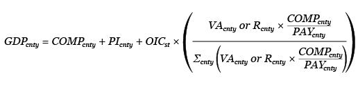
By a simple rearrangement of terms in equation 1, above, GDP can be computed as

Excluding compensation of employees and proprietors' income, all the other income payments and costs (OIC) can be represented by

With the exception of farming, mining, and government, BEA computes county-level GDP as the sum of COMP, the proprietors' income portion of gross operating surplus, and OIC.

The primary source data for the official GDP by county statistics include BEA county-level compensation and proprietors' income data. Compensation data are used in all industries except in farms, and proprietors' income data are used in all industry sectors except in mining and government. Additional data sources are used to distribute state-level OIC to counties. These data include National Establishment Time Series (NETS) sales data, Quarterly Census of Employment and Wages (QCEW) data, Economic Census data, and industry-specific data from various sources. Table 1 lists the different data sources used by published industry. Finally, BEA state and national GDP, compensation, and proprietors' income data are also incorporated to reconcile the regional estimates with national estimates.
| Industry | BEA county compensation | BEA county proprietors' Income | Economic Census | National Establishment Time Series | Additional source data |
|---|---|---|---|---|---|
| Agriculture, forestry, fishing, and hunting1 | ✓ | ✓ | ✓ | ||
| Mining1 | ✓ | ✓ | |||
| Utilities2 | ✓ | ✓ | ✓ | ||
| Construction2 | ✓ | ✓ | ✓ | ||
| Manufacturing | ✓ | ✓ | ✓ | ✓ | |
| Wholesale trade | ✓ | ✓ | ✓ | ✓ | |
| Retail trade | ✓ | ✓ | ✓ | ✓ | |
| Transportation and warehousing1 | ✓ | ✓ | ✓ | ✓ | ✓ |
| Information | ✓ | ✓ | ✓ | ✓ | |
| Finance and insurance1 | ✓ | ✓ | ✓ | ✓ | ✓ |
| Real estate and rental and leasing1 | ✓ | ✓ | ✓ | ✓ | ✓ |
| Professional, scientific, and technical services | ✓ | ✓ | ✓ | ✓ | |
| Management of companies and enterprises | ✓ | ✓ | |||
| Administrative and waste services | ✓ | ✓ | ✓ | ✓ | |
| Educational services | ✓ | ✓ | ✓ | ✓ | |
| Healthcare and social assistance | ✓ | ✓ | ✓ | ✓ | |
| Arts, entertainment, and recreation | ✓ | ✓ | ✓ | ✓ | |
| Accommodation and food services | ✓ | ✓ | ✓ | ✓ | |
| Other services, except government | ✓ | ✓ | ✓ | ✓ | |
| Government | ✓ | ✓ |
- Additional source data in the sub-industry detail.
- Additional source data at the sector level.
Although BEA publishes total GDP or value added by county for 21 distinct sectors, value added is estimated for the same 65 detailed industries found in the GDP by state accounts before being aggregated to the published industries. Except in the cases of farming, mining, and government, for each detailed industry, the state total of OIC is distributed to counties and then summed with BEA county compensation and proprietors' income to compute current-dollar county GDP by industry. National prices are then used to deflate current-dollar GDP values to obtain real (chained-dollar) GDP by county statistics.
Compensation of employees is the sum of wage and salary accruals and of supplements to wages and salaries. The county estimates of wages and salaries are based primarily on QCEW data that originate from the state unemployment insurance (UI) system and from the UI program for federal civilian employees. These data are assembled by the Bureau of Labor Statistics (BLS) of the U.S. Department of Labor. The data (reported quarterly on Form ES–202, the state UI contribution reports filed by employers in the industries covered by, and subject to, each state's UI laws and by federal agencies) are tabulated by county and by the North American Industry Classification System six-digit industry. The QCEW data account for 94.2 percent of wages and salaries estimated by BEA.2
In addition to the BLS QCEW data, BEA uses other data sources to estimate wages and salaries for a few industries that are partially covered or not covered by QCEW data. These industries include farms and agriculture and forestry support activities, which use U.S. Department of Agriculture (USDA) Census of Agriculture data; rail transportation, which uses Railroad Retirement Board payroll and employment data and Census Bureau Journey to Work (Census of Population) data; educational services, which use Census Bureau County Business Patterns and other county-specific data; and membership associations and organizations, which use household population data. Table 2 lists other additional industry-specific data sources used to estimate wages and salaries.
The data for employer contributions for employee pension and insurance funds portion of supplements to wages and salaries come from BEA estimates of wage and employment for all industries. For the employer contributions to government social insurance portion, BEA uses BLS state unemployment insurance programs' employer contribution data.
The estimates of proprietors' income are prepared in two parts—nonfarm proprietors' income and farm proprietors' income. Nonfarm proprietors' income accounted for approximately 97.7 percent of proprietors' income, while farm proprietors' income only accounted for approximately 2.3 percent in 2018. BEA uses IRS data on net profits of sole proprietorships and partnerships to estimate proprietors' income for all nonfarm industries, while using various data from USDA for farm proprietors' income.3 Table 2 also provides data sources used to estimate proprietors' income.
| Data | Source |
|---|---|
| Wages and salaries by industry | |
| In general | BLS Quarterly Census of Employment and Wages data |
| Farm | USDA Census of Agriculture data |
| Agriculture and forestry support activities | USDA Census of Agriculture data |
| Rail transportation | RRB payroll and employment data; Census Bureau Journey to Work (Census of Population) data |
| Educational services | Census Bureau County Business Patterns payroll data; state departments of education employment data; DOE Private School Universe Survey employment data; Official Catholic Directory number of teachers in religious orders data |
| Membership associations and organizations | Household population data |
| Private households | Household population data; Census Bureau Journey to Work (Census of Population) data |
| Military | DOD personnel data; DHS Coast Guard personnel and payroll data; household population data |
| State and local government | Census Bureau American Community Survey wage data; RRB payroll and employment data |
| Employer contributions for employee pension and insurance funds by industry | |
| All industries | BEA estimates of wages and employment |
| Employer contributions for government social insurance by industry | |
| All industries | BLS state unemployment insurance programs employer contributions data |
| Proprietors' income | |
| Farm | USDA Census of Agriculture data; USDA National Agriculture and Statistic Service crop production and livestock stocks data; cash receipts from state offices of agricultural statistics; USDA Farm Service Agency and Natural Resource Conservation Service government payments to farmers data; USDA Risk Management Agency crop indemnity payments data |
| Nonfarm industries | IRS data on net profits of sole proprietorships and partnerships |
- BEA
- Bureau of Economic Analysis
- BLS
- Bureau of Labor Statistics
- CMS
- Centers for Medicare and Medicaid Services
- DHS
- Department of Homeland Security
- DOD
- Department of Defense
- DOE
- Department of Education
- DVA
- Department of Veterans Affairs
- IRS
- Internal Revenue Service
- NSF
- National Science Foundation
- OPM
- Office of Personnel Management
- RRB
- Railroad Retirement Board
- SSA
- Social Security Administration
- USDA
- U.S. Department of Agriculture
Economic Census data are incorporated to estimate the OIC portion of county GDP in most of the detailed industries. The Economic Census is conducted every 5 years and captures data from roughly four million U.S. companies.4 It contains data from companies across the economic spectrum (large and small and goods-producing and services-producing companies) and is a critical source for many BEA statistical products. The GDP by county statistics rely heavily on this data. Value-added and payroll county data are used to distribute state OIC to counties for goods-producing industries, while receipts and payroll county data are used to distribute state OIC for services-producing industries. The majority (49 of 65) of the detailed industries estimated in the preparation of the GDP by county statistics are computed using Economic Census data.
The Census value added of manufacturing activity is derived by subtracting the cost of materials, supplies, containers, fuel, purchased electricity, and contract work from the value of shipments (products manufactured plus receipts for services rendered). The result of this calculation is adjusted by the addition of value added by merchandising operations (that is, the difference between the sales value and the cost of merchandise sold without further manufacture, processing, or assembly) plus the net change in finished goods and work-in-process between the beginning- and end-of-year inventories.
Census sales, value of shipments, or revenue refers to all appropriate dollar volume measures including total sales, value of shipments, revenue, receipts, or business done at any time during the year, whether or not payment was received during the year, by domestic establishments (excluding foreign subsidiaries) within the scope of the Economic Census.5
Both the Economic Census value added and receipts series are transformed by multiplying the corresponding series by the ratio of BEA compensation of employees to Economic Census payroll (equation 3); this is done to ensure consistency between the BEA income components and the Economic Census data, which are derived from different sample sets. The compensation-to-payroll ratio is used to adjust the coverage differences between the Economic Census and QCEW data used for the compensation estimates. This approach is consistent with the GDP by state approach. Equation 5, below, represents how GDP by county is estimated using Economic Census data.
Where:
GDPcnty = GDP by county
COMPcnty = GDP by county compensation of employees
PIcnty = GDP by county proprietors' income
OICst = GDP by state other income payments and costs
VAcnty = Economic Census county value added
Rcnty = Economic Census county receipts
PAYcnty = Economic Census county payroll
Years in which Economic Census data are available are considered benchmark years. Since the Census Bureau publishes the Economic Census every 5 years, in years when Economic Census data are not available, sales data from the NETS database are used to interpolate or extrapolate Economic Census values.
NETS is a time series database consisting of annual data from Dun & Bradstreet for over 59 million establishments from 1990 to 2015. The starting point for the NETS database is the annual snapshots of the full Duns Marketing Information (DMI) file. These snapshots use the DMI file to determine which establishments were active in each year in question. Other archival files (for example, the Credit Rating file) are utilized to provide annual raw establishment data. This collection of data includes a wealth of information on establishments, such as location, ownership structure, industrial operation structure, years of operation, relocation, industry classification, births and deaths, sales, and employment.
Industry-specific data. In contrast to general data sources, many of the data sources used to compute GDP by county statistics are specific to one industry. These data were chosen carefully based on availability, coverage, quality, and uniformity with other BEA accounts as well as the ability to better distribute state OIC to counties for a particular industry. In most cases, the county data are data from the same source as state data used for the GDP by state estimates. Table 3 lists the data sources and the industries that rely upon those data. A description of each industry and the data source(s) follows the table. For all the industries listed in table 3, except farms, the source data are used to generate county shares that are then used to distribute the state OIC to counties.
| Industry | Additional source data | Accessibility |
|---|---|---|
| Agriculture, forestry, fishing, and hunting | ||
| Farms | BEA farm income and expenses (cash receipts from marketings; imputed and miscellaneous income received; value of inventory change; production expenses) | Public |
| Mining | ||
| Oil and gas extraction | Oil and gas production data from DrillingEdge | Private |
| Mining except oil and gas extraction | Wages from BLS; EIA Annual Coal Report, tons of coal production | Public |
| Utilities | Net electricity generation data from EIA survey form EIA-923 Power Plant Operations Report | Public |
| Construction | Value put in place from Dodge Data & Analytics | Private |
| Transportation and warehousing | ||
| Air transportation | U.S. Airline Financial Data (Schedule P-1.2) and U.S Air Carrier Traffic Statistics (T-100 Domestic and International Segments) from BTS | Public |
| Rail transportation | DOT Surface Transportation Board Carload Waybill Sample | Public |
| Finance and insurance | ||
| Banking | Deposits by bank branch from FDIC Summary of Deposits Annual Survey of Branch Office Deposits | Public |
| Real estate and rental and leasing | ||
| Real estate | BEA imputed rent; BEA rental income from farms owned by nonoperator landlords; aggregate rent asked from the AHS | Public |
| Government | ||
| Federal civilian | Federal civilian and military employment from BLS; net electricity generation from EIA survey form EIA-923 Power Plant Operations Report; Postal Service wages from BLS | Public |
| Federal military | Federal military employment from BLS | Public |
- AHS
- American Housing Survey
- BEA
- Bureau of Economic Analysis
- BLS
- Bureau of Labor Statistics
- BTS
- Bureau of Transportation Statistics
- DOT
- U.S. Department of Transportation
- EIA
- Energy Information Agency
- FDIC
- Federal Deposit Insurance Corporation
Mining. The mining sector is composed of three industries—oil and gas extraction; mining (except oil and gas); and support activities for mining. Statistics for the mining sector incorporate oil and gas extraction volume of production data from DrillingEdge, oil and gas price data from the Energy Information Administration (EIA), coal production from EIA, wage data from BLS, wage data from BEA, and unpublished detail from the GDP by state accounts. The state OIC portion for the oil and gas extraction industry is distributed to counties by multiplying oil and gas volumes by county with regional price data used in the estimation of GDP by state. The state OIC portion of the mining except oil and gas industry is distributed to counties using coal production data from EIA and the noncoal portion of the industry is distributed using BLS wage data and unpublished GDP by state industry detail. OIC for support activities for mining are distributed to counties using BEA wages.
Utilities. The utilities sector includes electric power generation, transmission and distribution, natural gas distribution, water, sewage, and other systems. State data show that electricity generation is the primary driver of the utilities industry; therefore, data from EIA on net generation of electricity from power plants was chosen to distribute OIC to counties.
Construction. OIC for the construction sector is distributed to counties using construction spending data from Dodge Data & Analytics. These data reflect the value of construction projects that have been expended toward the completion of the project.
Transportation and warehousing. Two industries within the transportation and warehousing sector incorporate industry-specific data—air transportation and rail transportation. The data used in the state accounts to determine the place of performance are also available at the county level for both industries. OIC by state for the airline transportation industry is distributed to counties using airline revenue and passenger data from the Bureau of Transportation Statistics. BEA uses passenger enplanements, by company and airport, and airline financial data, by company, from the U.S. Department of Transportation.
For rail transportation, OIC by state is distributed to counties using tonnage and revenue waybill data from the U.S. Department of Transportation Surface Transportation Board. Revenue is apportioned in an equal split to the origination node and to the termination node.
State OIC for the rest of the transportation and warehousing sector is distributed to counties using Economic Census data, as discussed at the beginning of this section.
Finance and insurance. Four industries comprise the finance and insurance sector: banking, which includes monetary authorities-central bank, credit intermediation, and related services; securities, commodity contracts, and other financial investments and related activities; insurance carriers and related activities; and funds, trusts, and other financial vehicles. State OIC for the banking industry is distributed to counties with bank deposit data from the Federal Deposit Insurance Corporation (FDIC). The FDIC Summary of Deposits Survey publishes bank deposits by branch in each county for every active bank. The use of branch data enables a distribution series to be constructed that reflects where the activity takes place, rather than where banks are headquartered—a distinction that is important due to the prevalence of interstate branching. The other three industries in the finance and insurance sector use Economic Census to apportion OIC by county.
Real estate and rental and leasing. The real estate industry is one of two industries that comprise the real estate and rental and leasing sector. OIC by state is distributed to counties for the real estate industry using contract rent statistics from the Census Bureau American Housing Survey, imputed rent from BEA, wage data from BEA, farm rent statistics from BEA, and unpublished industry detail on housing services from the GDP by state estimates. Imputed rent for owner-occupied housing and mobile homes from BEA county personal income estimates is used to distribute the unpublished GDP by state totals for those types of housing services. Aggregate rent from the American Housing Survey is used to distribute the tenant-occupied housing portion.6 For other real estate, excluding owner-occupied and tenant-occupied rents, OIC by state is distributed to counties using Economic Census data. For the rental and leasing portion of the sector, OIC by state is distributed as well to counties using Economic Census data.
Government. The government sector includes federal military, federal civilian, and state and local governments. A significant portion of this sector's value added originates from compensation of employees, given the sector includes neither proprietors' income nor sizable portions of OIC such as TOPI or remaining portions of GOS like corporate profits. The OIC in this sector is primarily comprised of CFC and surplus or deficit of government enterprises. Unlike other sectors, the state OIC for government is calculated by just subtracting state compensation from the state GDP. State OIC is then apportioned to counties using various data sources and unpublished industry detail from the GDP by state estimates.
The OIC for federal military is distributed to counties using domestic troops employment data from BLS. For Federal civilian, which includes general government and federal enterprises such as federal power authorities, OIC is distributed to counties using federal civilian and military employment data from BLS, net electricity generation data from EIA for federal power authorities, postal service wages from BLS for postal service surplus or deficit, and BEA federal civilian wages and salaries. State-level OIC for state and local governments is distributed to counties using BEA wages and salaries data.
Agriculture, forestry, fishing, and hunting. The agriculture, forestry, fishing, and hunting sector includes two industries—forestry, fishing, and related activities and farms. State OIC for the forestry, fishing, and related activities industry is distributed to counties using QCEW data.
The farm industry is estimated differently than all other industries because of the availability of source data. The farm industry is not estimated as the sum of COMP, PI, and OIC. For the farm industry, GDP or value added by county is estimated directly using the production approach, in which GDP is measured as gross output minus intermediate inputs—the same methodology used in the estimation of GDP by state. Value added by county for farms is initially calculated using USDA data for farm income and farm expenses. Farm income is the sum of cash receipts, other farm income, and inventory change. Farm expenses include the purchase of the following goods and services: feed, livestock, seed, fertilizer and lime, petroleum products, veterinary services, pesticide, rental expense of nonoperator landlords, equipment operation and repair, electricity, and miscellaneous expenses. The difference between farm income and expenses is the initial estimate of gross output minus intermediate inputs. The initial county estimates are then scaled to the GDP by state estimates for the farming industry so that the county estimates reconcile to the state estimates.
Real GDP by county was prepared in chained (2012) dollars. Real GDP by county is an inflation-adjusted measure of each county based on national prices. These measures are important when making comparisons over time and when calculating growth.
The real statistics for each industry in each county are derived by applying national chain-type price indexes from the BEA Industry Economic Accounts to the statistics on current-dollar GDP by county for the detailed industries. For aggregate industry sectors and total GDP, real GDP by county statistics are derived by using the same chain-type index formula that is used in the national accounts.
To the extent that a county's output is produced and sold in national markets at relatively uniform prices (or sold locally at national prices), real GDP by county should accurately capture the relative differences in the mix of goods and services that counties produce. However, these statistics do not capture county-to-county differences in the prices that may exist locally for some goods and services.
- A sole proprietorship is an unincorporated business required to file Schedule C of Internal Revenue Service Form 1040 (Profit or Loss from Business) or Schedule F (Profit or Loss from Farming). A partnership is an unincorporated business association required to file Form 1065 (U.S. Return of Partnership Income). The dividends are included in personal dividend income, the monetary interest in personal interest income, and the rental income in rental income of persons.
- For more information on the estimation of county compensation, see “Local Area Personal Income Methodology” on the BEA website.
- For more information on the estimation of county proprietors' income, see “Local Area Personal Income Methodology.”
- For more information on the Economic Census, see “About the Economic Census” on the U.S. Census Bureau website.
- For more information on data definitions, see “Fields and Variables Glossary” on the Census website.
- The American Housing Survey (AHS) does not cover all counties for the entire time series. AHS 1-year data spans from 2005 to 2017, 3-year data from 2007 to 2013, and 5-year data from 2009 to 2017. These relevant data also exist in the 2000 decennial census. Moreover, only the 3- and 5-year files and the 2000 decennial census include all counties. Among these series, each county's data was selected at the greatest possible level of detail (3-year preferred to 5-year and 1-year preferred to either 3- or 5-year data). Census tract-level data from the 2000 decennial census were used to adjust county geographical definitions and values for new counties in Alaska and Colorado. The geometric mean of growth between 2000 and the earliest year available at the most detailed level were used to compute year 2001 values. From there, BEA series ”other monetary rental income of persons” was used as an indicator series to interpolate all remaining years missing from the AHS.