
Transactions of State and Local Government Defined Benefit Pension Plans
Experimental Estimates by State
State-level analysis of defined benefit pension plans for state and local government employees has long been hampered by an incomplete identification of the universe of public pension plans, changes in government accounting standards for pensions over time, and inconsistent economic assumptions and actuarial methods used by the pension plans. This article will describe the methods the Bureau of Economic Analysis (BEA) used to address these issues and provide an experimental set of state-level statistics describing the transactions of state and local government defined benefit pension plans. The set of statistics includes 32 series describing the current receipts, current expenditures, and cash flow of the pension plans as well as their assets and benefit entitlements. These current-dollar statistics display substantial regional variation.
BEA’s primary interest in developing this new data set is that some of the series currently are components of, or are used to estimate components of, state gross domestic product (GDP), state personal income, and state personal consumption expenditures on a place-of-work or place-of-residence basis. The other series require relatively little additional effort to estimate. Presenting the complete set of transactions of state and local government defined benefit pension plans in a separate table, all measured on a place of work basis, should enhance their usefulness to persons interested in public pensions.1
The estimates consist of a comprehensive set of annual transactions for 2000 to 2018, consistently measured on an accrual basis, using a common discount rate, and benchmarked to the 2017 Census of Governments. Such a complete set of state-level pension data is not available elsewhere and provides important data for public policy analyses and discussions.
This article will (1) describe the accounting framework used by BEA for defined benefit pension plans, (2) describe the state-level source data and estimation methodology, and (3) illustrate the use of the statistics in comparing defined benefit pension plans across states and across time. The new statistics show how the finances of the defined benefit plans have evolved over time and the effects of the Great Recession and subsequent recovery. In conjunction with their release, BEA is requesting comments on the statistics to assist in improving their quality, reliability, and usefulness. After taking account of the public comments, BEA intends to update the statistics annually as part of its state personal income statistics.
Retirement components of compensation of employees. Defined benefit pension plans are the largest, but not the only, retirement programs to which state and local governments contribute on behalf of their employees. They also contribute to defined contribution pension plans and to Social Security. Defined contribution plans are still relatively uncommon among state and local governments, but they are important in a few states, such as Alaska, Indiana, and Michigan. Most state and local governments also participate in Social Security, but in some states, such as Massachusetts and Ohio, very few governments participate. Actual employer contributions to defined benefit pension plans represented 76 percent of all state and local government contributions to retirement programs in 2018, employer contributions to Social Security were 18 percent, and employer contributions to defined contribution pension plans were 6 percent.
Importance of accrual accounting. Pension plans are a type of deferred compensation in which the employee agrees to future payments for work done in the current period. In national economic accounting, production and the income earned on that production should be recorded in the same period. Accrual accounting aligns the pension component of compensation with the period of service during which employees earned the benefits, reduces volatility in estimates of compensation arising from sporadic cash contributions to pension plans, and improves the accuracy of employers’ pension expenses when plans are overfunded or underfunded.
The state and local government defined benefit pension statistics will be published in a table similar to table 1, which displays data for New York for 2017 and 2018. The estimates in table 1 are an aggregation of all the defined benefit pension plans in New York—state administered plans as well as plans administered by New York City. This table is similar to table 7.24 in the National Income and Product Accounts (NIPAs). It uses an accounting framework based on the System of National Accounts 2008, which BEA adopted for the NIPAs in the 2013 comprehensive update. Lines 1–14 provide details on the current receipts of the pension plans, lines 15–21 provide details on the current expenditures, lines 22–26 provide details on the cash flow of the pension plans, and lines 27–32 are addenda (which are not in the NIPA table).
Current receipts. There are three major types of current receipts: output (line 2), contributions (line 3), and income receipts on assets (line10). The administrative expenses of the pension plan (called pension service charges on line 8) are subtracted from actual employer contributions (line 5) and recorded separately as output on line 2.
Contributions consist of claims to benefits accrued through service to employers (line 4) and household pension contribution supplements (line 9). In the public sector, it is typical for employees as well as employers to contribute to the funding of pensions. The employer portion is known as employers’ normal cost, and the employee portion is called actual household contributions (line 7). Employers’ normal cost (line 27) is broken down in this section of the table into actual employer contributions (line 5) plus imputed employer contributions (line 6) less pension service charges (line 8). Pension plan financial statements report actual employer contributions and pension service charges; imputed employer contributions is a balancing term that equates those items with employers’ normal cost.2 The imputed income payments on assets received by persons from the pension plans (line 17) are reinvested in the pension plan as household pension contribution supplements (line 9).
The third type of current receipt is income receipts on assets (including plans’ claims on employers) (line 10). These receipts consist of interest (line 11) and dividends (line 14). Monetary interest (line 12) and imputed interest on plans’ claims on employers (line 13) compose interest. Imputed interest can be positive or negative depending upon whether the plan is underfunded (the plan has a claim on the employer) or overfunded.
Current expenditures. Pension funds have four major types of current expenditures (line 15). Administrative expenses (line 16) have been discussed already. On line 17, the income receipts on assets of the pension plans (interest and dividends) are treated as if they were paid out to the household sector (where they show up in personal income) and then rerouted back to the pension fund sector as contribution supplements (line 9). In other words, pension funds are treated as “pass-through” entities that do not have income or saving on their own. Benefit payments and withdrawals are shown on line 20, and the net change in benefit entitlements is shown on line 21.
Cash flow. On a cash basis, the inflows of the pension plans are actual employer and household contributions (line 23) plus the monetary income receipts on assets (line 24). The outflows are benefit payments and withdrawals (line 25) and administrative expenses (line 26).
Estimates for New York. Public employees in New York accrued $20.1 billion in defined benefit pension benefits in 2018. They contributed $1.8 billion from their wages and salaries to fund these future benefits, and their government employers contributed $18.0 billion. Of those contributions, $2.4 billion were for the service charges of the pension plans. Since actual household and employer contributions net of pension service charges were less than claims to benefits accrued, BEA imputed $2.8 billion of employer contributions.
The claims to benefits accrued through service to employers can be put in perspective by noting that they amounted to 22.1 percent of the wages and salaries of state and local government employees in New York in 2018.3
Income receipts on assets were $25.6 billion for New York for 2018. Monetary interest and dividends accounted for $9.2 billion and $5.6 billion, respectively, and imputed interest on plans’ claims on employers was $10.8 billion.4 Plans’ claims on employers, recorded among the addenda (line 31), were $317.8 billion in 2018. This is the difference between benefit entitlements, which were $830.9 billion in 2018 (line 29), and pension plan assets, which were $513.2 billion (line 30). The funded ratio for New York in 2018 was 61.8 (line 32). In other words, New York pension plans had assets equal to 61.8 percent of the benefit entitlements.
Cash flow for the New York pension funds was negative in 2018, $3.0 billion. The inflows of actual employer and household contributions plus the monetary income receipts on assets were less than the outflows of benefit payments and administrative expenses. Benefit payments and withdrawals were $35.2 billion in New York in 2018.
Among the addenda to the table is interest accrued on benefit entitlements (line 28).5 It was $31.9 billion for New York in 2018. Employers’ normal cost (line 27) can be calculated as actual employer contributions plus imputed employer contributions less pension service charges, or equivalently, it can be calculated as claims to benefits accrued through service to employers less actual household contributions. It was $18.4 billion for New York in 2018. Because of its importance as a part of the compensation of employees, and because it varies widely across states, it is reported separately in the addenda to the table.
| Line | Description | 2017 | 2018 |
|---|---|---|---|
| 1 | Current receipts, accrual basis | 74,061 | 73,755 |
| 2 | Output | 2,101 | 2,364 |
| 3 | Contributions | 46,297 | 45,752 |
| 4 | Claims to benefits accrued through service to employers | 20,635 | 20,113 |
| 5 | Actual employer contributions | 18,028 | 17,966 |
| 6 | Imputed employer contributions | 2,942 | 2,752 |
| 7 | Actual household contributions | 1,767 | 1,759 |
| 8 | Less: Pension service charges | 2,101 | 2,364 |
| 9 | Household pension contribution supplements1 | 25,662 | 25,639 |
| 10 | Income receipts on assets (including plans' claims on employers) | 25,662 | 25,639 |
| 11 | Interest | 20,084 | 20,079 |
| 12 | Monetary interest | 7,899 | 9,239 |
| 13 | Imputed interest on plans' claims on employers2 | 12,185 | 10,839 |
| 14 | Dividends | 5,578 | 5,560 |
| 15 | Current expenditures, accrual basis | 74,061 | 73,755 |
| 16 | Administrative expenses | 2,101 | 2,364 |
| 17 | Imputed income payments on assets to persons | 25,662 | 25,639 |
| 18 | Interest | 20,084 | 20,079 |
| 19 | Dividends | 5,578 | 5,560 |
| 20 | Benefit payments and withdrawals | 33,498 | 35,168 |
| 21 | Net change in benefit entitlements3 | 12,799 | 10,583 |
| 22 | Cash flow | −2,327 | −3,008 |
| 23 | Actual employer and household contributions | 19,795 | 19,725 |
| 24 | Monetary income receipts on assets | 13,477 | 14,800 |
| 25 | Less: Benefit payments and withdrawals | 33,498 | 35,168 |
| 26 | Less: Administrative expenses | 2,101 | 2,364 |
| Addenda: | |||
| 27 | Employers' normal cost | 18,869 | 18,354 |
| 28 | Interest accrued on benefit entitlements | 30,955 | 31,908 |
| 29 | Benefit entitlements | 805,157 | 830,921 |
| 30 | Pension plan assets | 534,171 | 513,169 |
| 31 | Plans' claims on employers | 270,986 | 317,751 |
| 32 | Funded ratio4 | 66.3 | 61.8 |
- Imputed income payments received by persons from the pension plans (line 17) are reinvested as household pension contribution supplements.
- Plans' claims on employers is the difference between benefit entitlements and assets held by plans. When benefit entitlements exceed plan assets, imputed interest is positive; when plan assets exceed benefit entitlements, imputed interest is negative.
- Excludes implied funding of benefits from holding gains on assets and excludes effects on change in the estimated value of benefit entitlements that come from differences between actual experience and previous actuarial assumptions, changes in actuarial assumptions, and changes in plan provisions.
- The funded ratio is pension plan assets divided by benefit entitlements times 100.
Note. The effects of participation in defined benefit pension plans on state personal income and state personal consumption expenditures requires that the estimates in this table be adjusted for the residence of the members of the plans and are not shown.
| Years | Discount rate |
|---|---|
| 2000–2003 | 6.0 |
| 2004–2009 | 5.5 |
| 2010–2012 | 5.0 |
| 2013–2018 | 4.0 |
The new state-level pension estimates are useful for comparing states at a given point in time and for observing how they have changed since 2000. The pension liabilities do not represent the legal liability of any particular government, but they are useful for studying the macroeconomic implications of aggregated public sector defined benefit pension plans. They are useful for discussion of public policies regarding unfunded liabilities and compensation of state and local government employees. The statistics display substantial state-level variation.
BEA discount rate. The actuarial estimates in the new set of pension statistics are based on a discount rate that is the same for every state but changes over time.6 The discount rate was 6 percent for 2000 to 2003, 5.5 percent for 2004 to 2009, 5 percent for 2010 to 2012, and 4 percent from 2013 to 2018 (table 2).
Funded ratio. Benefit entitlements in 2018 ranged from $1,857.3 billion in California to $10.5 billion in Vermont (table 3). Such a ranking tells one little more than Vermont is a smaller state than California and by how much. More informative is the funded ratio, which compares benefit entitlements to the resources available to the pension funds. The funded ratio in 2018 ranged from 69.3 percent for South Dakota to 28.2 percent for New Jersey (table 4). The funded ratios of most states fell sharply on two occasions since 2000, reflecting bear markets from 2000 to 2002 after the dot-com bust, and from 2007 to 2008 after the financial crisis (chart 1). South Dakota’s and New Jersey’s funded ratios declined 16.5 and 15.0 percentage points, respectively, in the first bear market and 24.1 and 10.5 percentage points in the second. In the 10 years since the financial crisis of 2008, South Dakota’s funded ratio rose 11.5 percentage points, while New Jersey’s funded ratio fell another 4.0 percentage points. Since 2008, the U.S. funded ratio has fluctuated in a narrow band around 49 percent. The negative cash flow that most plans face today makes it difficult to return to the funding ratio of nearly 76.5 percent before the financial crisis. In 2018, pension plan cash flow was negative for 38 states, up from 3 states in 2000 (table 5).

[Click chart to expand]
Ratio of benefit entitlements to personal income. Another useful ratio is benefit entitlements relative to a measure of the size of the state economy, such as personal income or GDP (both ratios tend to move together). Benefit entitlements as a percentage of state personal income ranged from 79.3 percent in Alaska to 19.9 percent in Indiana in 2018 (table 6). Since 2000, benefit entitlements have grown from 35.3 percent of personal income to 48.4 percent for the United States (chart 2). Some of the increase represents reductions in the BEA discount rate, but from 2013 to 2018, the rate was unchanged. From 2013 to 2018, U.S. benefit entitlements grew at a slightly slower pace than personal income. In North Dakota, benefit entitlements rose from 25.8 percent to 32.8 percent of personal income from 2013 to 2018, while in New Jersey benefit entitlements fell from 45.6 percent to 42.7 percent over the last 5 years (chart 2).

[Click chart to expand]
Claims to benefits accrued through service to employers, relative to wages and salaries of state and local government employees. A crucial variable driving the growth in benefit entitlements is claims to benefits accrued through service to employers. Up to now, that information has not been available as a time series measured consistently across states using a common discount rate. Claims to benefits accrued through service to employers as a percentage of the wages and salaries of all state and local government employees was highest in California in 2018 (33.2 percent), followed by Nevada (32.2 percent) and Illinois (31.3 percent). Indiana (6.8 percent) and Michigan (10.1 percent) were lowest (table 7).7
For the United States, this ratio rose only 2 percentage points, from 19.7 percent in 2000 to 21.8 percent in 2018 (chart 3). (The upticks in the chart correspond to reductions in the BEA discount rate.) In contrast, California’s rate rose substantially from 25.0 percent in 2000 to 33.2 percent in 2018, while Indiana fell from 9.0 percent in 2000 to 6.8 percent in 2018. Indiana’s state-administered plans have two components: one is a defined benefit plan funded by employer contributions, and the other is a defined contribution plan funded by employee contributions. In most other states, the contributions of both employers and employees are used to fund only the defined benefit plan.

[Click chart to expand]
Actual household contributions. One response to low pension plan funded ratios has been to require active employees to contribute more to the funding of their pensions, that is, to increase actual household contributions. As a percentage of the wages and salaries of all state and local government employees, these contributions ranged from 10.9 percent in Ohio and 8.9 percent in Massachusetts to 0.1 percent in Oregon and 0.4 percent in Indiana in 2018 (table 8). The national average was 5.7 percent in 2018, up from 4.5 percent in 2008. The biggest increases were in Virginia, up 3.8 percentage points, and North Dakota, up 2.5 percentage points (chart 4). The low rates in Oregon and Indiana reflect the fact that most employee contributions are placed in defined contribution plans.

[Click chart to expand]
Actual employer contributions relative to employers’ normal cost. Employers’ normal cost is the employers’ share of the claims to benefits accrued through service to employers. Funding shortfalls occur when actual employer contributions less pension service charges are less than employers’ normal cost, as was the case in Illinois from 2000 to 2016 (chart 5). In contrast, since at least 2000, West Virginia has been making catch-up contributions in excess of employers’ normal cost (chart 6). Sustained underfunding of pensions (as in the case of Illinois) or sustained catch-up contributions (in the case of West Virginia) make a difference to the funded ratio. In 2000, West Virginia had the lowest funded ratio in the nation, 38.8 percent (Illinois was 53.9 percent). By 2018, West Virginia had increased its funded ratio to 53.7 percent, while Illinois’ funded ratio had fallen to 29.8 percent (chart 7).

[Click chart to expand]

[Click chart to expand]

[Click chart to expand]
The size of current funding shortfalls is measured by imputed employer contributions (table 9). In 2018, imputed employer contributions were positive in 37 states and negative in 13. (Positive values indicate funding shortfalls, and negative values represent catch-up payments for contribution shortfalls in the past and the interest thereon.)
| State | 2018 entitlements | Rank |
|---|---|---|
| Alabama | 84,131 | 28 |
| Alaska | 34,763 | 39 |
| Arizona | 115,702 | 22 |
| Arkansas | 57,771 | 34 |
| California | 1,857,266 | 1 |
| Colorado | 141,506 | 18 |
| Connecticut | 119,934 | 21 |
| Delaware | 18,120 | 46 |
| District of Columbia | 14,833 | ..... |
| Florida | 348,330 | 6 |
| Georgia | 210,131 | 9 |
| Hawaii | 44,962 | 37 |
| Idaho | 26,941 | 41 |
| Illinois | 563,228 | 3 |
| Indiana | 62,797 | 31 |
| Iowa | 62,031 | 32 |
| Kansas | 47,683 | 36 |
| Kentucky | 96,247 | 25 |
| Louisiana | 105,397 | 23 |
| Maine | 24,247 | 44 |
| Maryland | 157,623 | 15 |
| Massachusetts | 205,489 | 11 |
| Michigan | 208,082 | 10 |
| Minnesota | 131,165 | 19 |
| Mississippi | 70,184 | 29 |
| Missouri | 152,238 | 17 |
| Montana | 25,080 | 43 |
| Nebraska | 35,156 | 38 |
| Nevada | 85,745 | 27 |
| New Hampshire | 20,667 | 45 |
| New Jersey | 259,863 | 8 |
| New Mexico | 63,930 | 30 |
| New York | 830,921 | 2 |
| North Carolina | 158,718 | 14 |
| North Dakota | 13,828 | 49 |
| Ohio | 355,166 | 5 |
| Oklahoma | 59,389 | 33 |
| Oregon | 129,160 | 20 |
| Pennsylvania | 261,530 | 7 |
| Rhode Island | 26,588 | 42 |
| South Carolina | 87,915 | 26 |
| South Dakota | 17,553 | 47 |
| Tennessee | 98,455 | 24 |
| Texas | 526,110 | 4 |
| Utah | 52,349 | 35 |
| Vermont | 10,488 | 50 |
| Virginia | 173,705 | 12 |
| Washington | 159,740 | 13 |
| West Virginia | 28,887 | 40 |
| Wisconsin | 156,345 | 16 |
| Wyoming | 16,117 | 48 |
| United States | 8,614,206 | ..... |
Note. Rankings do not include the District of Columbia.
| State | Percent funded in 2018 | Rank |
|---|---|---|
| Alabama | 44.0 | 31 |
| Alaska | 41.2 | 38 |
| Arizona | 44.0 | 30 |
| Arkansas | 50.0 | 21 |
| California | 46.8 | 26 |
| Colorado | 37.5 | 43 |
| Connecticut | 36.6 | 44 |
| Delaware | 56.6 | 10 |
| District of Columbia | 58.6 | ..... |
| Florida | 53.6 | 13 |
| Georgia | 47.4 | 25 |
| Hawaii | 35.5 | 45 |
| Idaho | 59.1 | 4 |
| Illinois | 29.8 | 49 |
| Indiana | 45.1 | 29 |
| Iowa | 54.7 | 11 |
| Kansas | 42.6 | 34 |
| Kentucky | 32.8 | 48 |
| Louisiana | 48.1 | 24 |
| Maine | 56.9 | 9 |
| Maryland | 45.5 | 28 |
| Massachusetts | 38.7 | 42 |
| Michigan | 41.7 | 36 |
| Minnesota | 50.7 | 18 |
| Mississippi | 38.8 | 41 |
| Missouri | 48.6 | 22 |
| Montana | 43.8 | 32 |
| Nebraska | 51.1 | 17 |
| Nevada | 45.7 | 27 |
| New Hampshire | 41.9 | 35 |
| New Jersey | 28.2 | 50 |
| New Mexico | 42.8 | 33 |
| New York | 61.8 | 3 |
| North Carolina | 58.5 | 6 |
| North Dakota | 40.1 | 39 |
| Ohio | 50.2 | 19 |
| Oklahoma | 52.4 | 14 |
| Oregon | 51.9 | 16 |
| Pennsylvania | 39.4 | 40 |
| Rhode Island | 35.3 | 46 |
| South Carolina | 33.7 | 47 |
| South Dakota | 69.3 | 1 |
| Tennessee | 58.6 | 5 |
| Texas | 50.1 | 20 |
| Utah | 58.0 | 7 |
| Vermont | 41.5 | 37 |
| Virginia | 52.3 | 15 |
| Washington | 57.3 | 8 |
| West Virginia | 53.7 | 12 |
| Wisconsin | 69.1 | 2 |
| Wyoming | 48.3 | 23 |
| United States | 47.3 | ..... |
Note. Rankings do not include the District of Columbia.
| State | 2000 | 2018 |
|---|---|---|
| Alabama | 959 | −464 |
| Alaska | 169 | −421 |
| Arizona | 266 | −596 |
| Arkansas | 465 | −606 |
| California | 7,832 | 10,390 |
| Colorado | 469 | −1,586 |
| Connecticut | 384 | −256 |
| Delaware | 150 | −192 |
| District of Columbia | 225 | 159 |
| Florida | 3,231 | −2,872 |
| Georgia | 2,271 | −730 |
| Hawaii | −115 | 165 |
| Idaho | 178 | 153 |
| Illinois | 2,308 | −1,889 |
| Indiana | 681 | −217 |
| Iowa | 360 | −209 |
| Kansas | 90 | −100 |
| Kentucky | 847 | −137 |
| Louisiana | 588 | −448 |
| Maine | 53 | −309 |
| Maryland | 728 | 1,152 |
| Massachusetts | 1,570 | 107 |
| Michigan | 649 | −1,886 |
| Minnesota | −183 | −721 |
| Mississippi | 565 | −656 |
| Missouri | 926 | −847 |
| Montana | 289 | 315 |
| Nebraska | 216 | 62 |
| Nevada | 645 | 212 |
| New Hampshire | 33 | −16 |
| New Jersey | 851 | −2,642 |
| New Mexico | 493 | −536 |
| New York | −935 | −3,008 |
| North Carolina | 1,323 | −290 |
| North Dakota | 98 | 93 |
| Ohio | 2,092 | −1,959 |
| Oklahoma | 350 | −96 |
| Oregon | 1,263 | −1,003 |
| Pennsylvania | 902 | −1,888 |
| Rhode Island | 150 | −239 |
| South Carolina | 1,100 | −815 |
| South Dakota | 134 | −43 |
| Tennessee | 1,168 | −45 |
| Texas | 4,579 | −14 |
| Utah | 550 | 265 |
| Vermont | 81 | 40 |
| Virginia | 1,088 | −223 |
| Washington | 731 | 2,660 |
| West Virginia | 105 | −430 |
| Wisconsin | 1,089 | −1,596 |
| Wyoming | 114 | −116 |
| United States | 44,176 | −14,328 |
| State | 2018 | Rank |
|---|---|---|
| Alabama | 40.8 | 26 |
| Alaska | 79.3 | 1 |
| Arizona | 36.4 | 34 |
| Arkansas | 44.3 | 18 |
| California | 73.9 | 3 |
| Colorado | 42.5 | 23 |
| Connecticut | 43.9 | 19 |
| Delaware | 35.7 | 37 |
| District of Columbia | 25.7 | ..... |
| Florida | 32.7 | 44 |
| Georgia | 43.0 | 21 |
| Hawaii | 57.1 | 10 |
| Idaho | 35.0 | 39 |
| Illinois | 77.8 | 2 |
| Indiana | 19.9 | 50 |
| Iowa | 39.2 | 29 |
| Kansas | 31.8 | 46 |
| Kentucky | 50.7 | 13 |
| Louisiana | 48.9 | 15 |
| Maine | 37.0 | 32 |
| Maryland | 41.2 | 25 |
| Massachusetts | 41.5 | 24 |
| Michigan | 43.0 | 20 |
| Minnesota | 40.6 | 27 |
| Mississippi | 62.1 | 6 |
| Missouri | 52.0 | 12 |
| Montana | 49.7 | 14 |
| Nebraska | 34.2 | 40 |
| Nevada | 57.5 | 9 |
| New Hampshire | 24.9 | 49 |
| New Jersey | 42.7 | 22 |
| New Mexico | 73.3 | 4 |
| New York | 61.9 | 7 |
| North Carolina | 33.1 | 42 |
| North Dakota | 32.8 | 43 |
| Ohio | 62.3 | 5 |
| Oklahoma | 32.6 | 45 |
| Oregon | 60.6 | 8 |
| Pennsylvania | 36.3 | 35 |
| Rhode Island | 45.8 | 17 |
| South Carolina | 39.6 | 28 |
| South Dakota | 38.1 | 31 |
| Tennessee | 31.0 | 47 |
| Texas | 36.4 | 33 |
| Utah | 35.8 | 36 |
| Vermont | 30.9 | 48 |
| Virginia | 35.3 | 38 |
| Washington | 34.2 | 41 |
| West Virginia | 39.1 | 30 |
| Wisconsin | 52.1 | 11 |
| Wyoming | 46.2 | 16 |
| United States | 48.4 | ..... |
Note. Rankings do not include the District of Columbia.
| State | 2018 claims | Rank |
|---|---|---|
| Alabama | 17.2 | 26 |
| Alaska | 18.3 | 23 |
| Arizona | 30.9 | 4 |
| Arkansas | 16.0 | 31 |
| California | 33.2 | 1 |
| Colorado | 13.1 | 46 |
| Connecticut | 21.2 | 14 |
| Delaware | 13.9 | 44 |
| District of Columbia | 16.2 | ..... |
| Florida | 11.6 | 48 |
| Georgia | 19.0 | 20 |
| Hawaii | 22.6 | 10 |
| Idaho | 20.4 | 16 |
| Illinois | 31.3 | 3 |
| Indiana | 6.8 | 50 |
| Iowa | 16.8 | 29 |
| Kansas | 15.0 | 40 |
| Kentucky | 16.2 | 30 |
| Louisiana | 21.4 | 13 |
| Maine | 15.8 | 32 |
| Maryland | 19.9 | 18 |
| Massachusetts | 27.0 | 5 |
| Michigan | 10.1 | 49 |
| Minnesota | 19.8 | 19 |
| Mississippi | 19.9 | 17 |
| Missouri | 21.0 | 15 |
| Montana | 18.9 | 21 |
| Nebraska | 15.5 | 37 |
| Nevada | 32.2 | 2 |
| New Hampshire | 14.4 | 43 |
| New Jersey | 15.3 | 38 |
| New Mexico | 22.2 | 11 |
| New York | 22.1 | 12 |
| North Carolina | 17.2 | 25 |
| North Dakota | 17.0 | 27 |
| Ohio | 24.2 | 6 |
| Oklahoma | 14.8 | 41 |
| Oregon | 17.7 | 24 |
| Pennsylvania | 23.6 | 8 |
| Rhode Island | 13.4 | 45 |
| South Carolina | 15.5 | 36 |
| South Dakota | 15.7 | 33 |
| Tennessee | 15.7 | 34 |
| Texas | 23.3 | 9 |
| Utah | 15.1 | 39 |
| Vermont | 12.5 | 47 |
| Virginia | 16.9 | 28 |
| Washington | 15.7 | 35 |
| West Virginia | 14.7 | 42 |
| Wisconsin | 23.8 | 7 |
| Wyoming | 18.7 | 22 |
| United States | 21.6 | ..... |
Note. Rankings do not include the District of Columbia.
| State | 2018 contributions | Rank | Change in contributions 2008–2018 | Rank |
|---|---|---|---|---|
| Alabama | 5.8 | 23 | 1.1 | 26 |
| Alaska | 3.6 | 40 | −2.3 | 49 |
| Arizona | 8.1 | 5 | 1.2 | 22 |
| Arkansas | 3.2 | 41 | 0.9 | 29 |
| California | 8.2 | 4 | 1.7 | 10 |
| Colorado | 5.1 | 30 | 0.4 | 38 |
| Connecticut | 5.3 | 27 | 2.1 | 3 |
| Delaware | 2.7 | 43 | 0.6 | 32 |
| District of Columbia | 2.5 | ..... | 0.1 | ..... |
| Florida | 2.4 | 45 | 1.6 | 12 |
| Georgia | 4.1 | 39 | 1.0 | 28 |
| Hawaii | 5.5 | 24 | 1.5 | 15 |
| Idaho | 6.0 | 19 | 1.1 | 24 |
| Illinois | 7.4 | 6 | 0.5 | 35 |
| Indiana | 0.4 | 49 | 0.1 | 43 |
| Iowa | 4.9 | 32 | 1.6 | 13 |
| Kansas | 5.0 | 31 | 1.5 | 14 |
| Kentucky | 6.4 | 14 | 0.5 | 34 |
| Louisiana | 6.3 | 16 | 0.4 | 39 |
| Maine | 5.8 | 21 | 1.1 | 25 |
| Maryland | 5.3 | 26 | 1.8 | 9 |
| Massachusetts | 8.9 | 2 | 0.6 | 33 |
| Michigan | 2.7 | 42 | 0.4 | 37 |
| Minnesota | 6.4 | 13 | 1.7 | 11 |
| Mississippi | 6.9 | 9 | 1.2 | 21 |
| Missouri | 6.8 | 10 | 1.4 | 18 |
| Montana | 6.8 | 11 | 0.7 | 31 |
| Nebraska | 5.2 | 29 | 1.4 | 17 |
| Nevada | 1.9 | 47 | 0.0 | 44 |
| New Hampshire | 6.2 | 17 | 1.5 | 16 |
| New Jersey | 6.4 | 12 | 1.1 | 23 |
| New Mexico | 8.5 | 3 | 2.1 | 4 |
| New York | 1.9 | 46 | 0.0 | 45 |
| North Carolina | 4.6 | 33 | 0.1 | 42 |
| North Dakota | 6.3 | 15 | 2.5 | 2 |
| Ohio | 10.9 | 1 | 1.4 | 20 |
| Oklahoma | 4.2 | 37 | −0.1 | 47 |
| Oregon | 0.1 | 50 | 0.0 | 46 |
| Pennsylvania | 5.8 | 22 | 0.7 | 30 |
| Rhode Island | 4.6 | 34 | −2.4 | 50 |
| South Carolina | 7.2 | 8 | 2.0 | 5 |
| South Dakota | 5.5 | 25 | 0.3 | 41 |
| Tennessee | 2.7 | 44 | 0.4 | 36 |
| Texas | 7.3 | 7 | 2.0 | 6 |
| Utah | 0.5 | 48 | −0.2 | 48 |
| Vermont | 5.2 | 28 | 2.0 | 7 |
| Virginia | 4.5 | 35 | 3.8 | 1 |
| Washington | 4.3 | 36 | 1.4 | 19 |
| West Virginia | 4.1 | 38 | 0.3 | 40 |
| Wisconsin | 6.2 | 18 | 1.1 | 27 |
| Wyoming | 6.0 | 20 | 1.9 | 8 |
| United States | 5.6 | ..... | 1.1 | ..... |
Note. Rankings do not include the District of Columbia.
| State | 2018 |
|---|---|
| Alabama | 435 |
| Alaska | 13 |
| Arizona | 2,033 |
| Arkansas | 217 |
| California | 2,698 |
| Colorado | 26 |
| Connecticut | −995 |
| Delaware | 107 |
| District of Columbia | 220 |
| Florida | 285 |
| Georgia | 713 |
| Hawaii | 103 |
| Idaho | 286 |
| Illinois | −1,640 |
| Indiana | −805 |
| Iowa | 583 |
| Kansas | 100 |
| Kentucky | −1,382 |
| Louisiana | −544 |
| Maine | −3 |
| Maryland | 361 |
| Massachusetts | 729 |
| Michigan | −2,222 |
| Minnesota | 1,301 |
| Mississippi | 206 |
| Missouri | 310 |
| Montana | 107 |
| Nebraska | 276 |
| Nevada | 797 |
| New Hampshire | −82 |
| New Jersey | −1,213 |
| New Mexico | 295 |
| New York | 2,752 |
| North Carolina | 1,769 |
| North Dakota | 103 |
| Ohio | 842 |
| Oklahoma | 121 |
| Oregon | 978 |
| Pennsylvania | −1,778 |
| Rhode Island | −304 |
| South Carolina | −104 |
| South Dakota | 131 |
| Tennessee | 812 |
| Texas | 6,870 |
| Utah | 221 |
| Vermont | −28 |
| Virginia | 403 |
| Washington | 764 |
| West Virginia | −149 |
| Wisconsin | 2,012 |
| Wyoming | 222 |
| United States | 18,952 |
We used two basic data sets for the state-level defined benefit pension estimates. For benefit entitlements and employers’ normal cost, we used data compiled by BEA from the financial statements of the pension plans (table 10).8 For the other estimates, we used data from the Census of Governments (for years ending in 2 and 7) and the Census Bureau’s Annual Survey of Public Pensions for intercensal years (table 11).
We used data from an edited version of the Census Bureau’s individual unit file. Editing entailed (1) replacement of missing values by interpolation or imputation, (2) replacement of outliers with values reported in pension plan financial statements, (3) extrapolation of data back to 1997 for pension plans discovered in more recent census years, (4) removal of out-of-scope plans, such as for volunteer firemen,9 (5) removal of deposits of the proceeds of pension obligation bonds from employer contributions, and (6) augmentation of the latest census with data for several large overlooked pension plans using data published in their financial statements.
State-level estimates based on the Census Bureau data were controlled to national estimates from the NIPAs, after conversion from fiscal years to calendar years.10 Calendar year estimates of pension plan assets were controlled to national estimates from the Financial Accounts of the United States produced by the Federal Reserve Board. The national sum of the edited individual unit file data was quite similar to the national controls, except for monetary interest, which was only 58 percent of the national control in 2017 (table 12). Many pension plans do not break down income receipts on assets into monetary interest and dividends in their financial statements, and some do not even report total income receipts on assets separately from other investment income, especially in recent years.11
The estimates are by the place of work of the active members of the pension plans, which is generally the same as the state in which the sponsoring government is located. However, the data for the Washington Metropolitan Area Transit Authority plans were allocated to the District of Columbia, Maryland, and Virginia, where it has worksites, on the basis of Quarterly Census of Employment and Wages (QCEW) data.12 Since the data are by place of work, employers’ normal cost and pension service charges can be directly compared to BEA estimates of employee compensation by state, which are also by place of work. In fact, employers’ normal cost and pension service charges are components of compensation.
Estimates for the income receipts on assets must be adjusted for the residence of both active members and beneficiaries of the plans before they can be compared to state estimates of personal dividend income and personal interest income. Similarly, pension service charges must be adjusted for residence of the plan members before they can be compared to state personal consumption expenditures.
Among the challenges to making state-level estimates of defined benefit pension transactions are (1) changes in government accounting standards over time, (2) standardizing the actuarial estimates on a common discount rate and actuarial cost method, (3) identifying the universe of pension plans, and (4) benchmarking the data to the 2017 Census of Governments.
Changes in government accounting standards over time. Relying on actuarial data reported by the pension plans, BEA estimated benefit entitlements and employers’ normal cost for the years 2000 to 2018. Preparing a similar set of estimates for earlier years is more difficult for several reasons, not least of which is the unsettled nature of pension accounting for state and local governments before generally accepted accounting practice settled on Statement No. 25 of the Governmental Accounting Standards Board (GASB 25).13 GASB 25 was effective for fiscal years beginning after June 15, 1996. Major changes to pension accounting were introduced in GASB 67, which was effective for fiscal years beginning after June 15, 2013. Fortunately, for most of the pension plans, we were able to obtain actuarial data compiled on both a GASB 25 and GASB 67 basis for fiscal year 2014. That enabled us to link estimates reported under the different accounting standards.
GASB 25. Under GASB 25, defined benefit pension plans (1) generally did not report the normal cost of the pension plan in their financial statements, (2) could choose one of six actuarial cost methods, and (3) could discount their liabilities using their investment rate of return. This reporting leeway is problematical because the magnitudes of the normal cost and the actuarial liability can vary substantially depending on which actuarial cost method is used to calculate them and which discount rate is used. In 2000, discount rates ranged from 5.75 percent (used by the Wisconsin Retirement System) to 9.00 percent (used by the Arizona Public Safety plan). The liability-weighted average discount rate of the plans in the BEA subset was 8.02 percent (table 13).
The first problem was solved by estimating normal cost from data published in the actuarial valuation reports of the pension plans.14 The second and third problems were solved by standardizing the data collected from the various pension plans on a common actuarial cost method (entry age) and discount rate in a manner similar to that described by Novy-Marx and Rauh (2011).15, 16
BEA compiled the data listed in table 10 for 120 of the largest state and local government defined benefit pension plans (the plans for which BEA compiled data will be referred to as the BEA subset). The liabilities and employers’ normal cost were adjusted from the plan discount rate and actuarial cost method to an estimate based on a 6 percent discount rate and the entry age cost method, plan by plan. Next, fiscal year estimates were converted to calendar year estimates. Next, the calendar year estimates were adjusted to the BEA discount rate. Then the plan-level estimates of employers’ normal cost and the active member liability were scaled up to the state level using the ratio of active members in all plans in the state to active membership in the BEA subset for the state. The plan-level estimates of the retired and beneficiary liabilities were scaled up using a similar ratio for retired and beneficiary members.
Next, the GASB 25 estimates were linked to the GASB 67 estimates by multiplying the former estimates by a ratio of the GASB 67 estimate for 2014 to the GASB 25 estimate for 2014. Lastly, the state estimates were adjusted proportionately so that they summed to the national control from the NIPAs.
GASB 67. As noted, GASB 67 was effective for fiscal years beginning after June 15, 2013. BEA compiled the items in table 10 from the pension plan financial statements for approximately 180 of the largest pension plans. The 50 percent increase over the size of the GASB 25 subset was necessitated by the loss of several agent multiple-employer pension plans and their replacement by smaller plans to keep the coverage above 75 percent for most states.17
GASB 67 improved the quality of the actuarial data presented in the financial statements of state and local government pension plans in three important respects. Pension plans are now required to report service cost (normal cost) and the sensitivity of the pension liability to changes in the discount rate. In addition, all pension plans are required to use the entry age actuarial cost method.
The total pension liability and the service cost reported by the pension plans in their financial statements continue to be based on discount rates that vary from plan to plan. In order to make the liabilities and service costs comparable across plans, BEA adjusted them to reflect a common discount rate. The adjustment of pension liabilities is given by
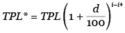
where TPL is the total pension liability reported by the pension plan based on the plan discount rate i and TPL* is the liability based on the BEA discount rate i*. The adjustment depends on duration d, which can be calculated as
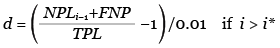
where NPLi-1 is the net pension liability at the plan discount rate less 1 percentage point (as reported by the pension plan), and FNP is the plan fiduciary net position at the end of the fiscal year. When the plan discount rate is lower than the BEA discount rate, duration can be calculated as
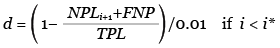
where NPLi+1 is the net pension liability at the plan discount rate plus 1 percentage point. Using data for fiscal year 2017 from the edited Census of Governments for 1,646 pension plans, the liability-weighted duration (for reductions in the discount rate) varied from 14.4 for Minnesota to 9.0 for Arizona; the national average was 12.5 (table 14).18
Since pension plans do not report similar interest rate data for employers’ normal cost, we continued to adjust employers’ normal cost for the BEA subset to the BEA discount rate using the method developed for the GASB 25 data described above. Liabilities were converted, plan by plan, to the BEA discount rate using equation 1. Next, the plan-level estimates of liabilities and employers’ normal cost were scaled up to the state level by the ratio of active, retired, and beneficiary membership of all plans in the state to membership in the BEA subset for the state (for liabilities) and the ratio of active membership of all plans in the state to membership in the BEA subset for the state (for employers’ normal cost). In addition, liabilities were benchmarked to an estimate based on data collected in the 2017 Census of Governments. Next, the fiscal year data for years t-1 and t were converted to calendar year t using equal weights for state plans and weights of 0.67 and 0.33, respectively, for local plans.19 Lastly, the state estimates were adjusted proportionately so that they summed to the national control from the NIPAs.20
Identifying the universe of pension plans. In the 1997 Census of Governments, the Census Bureau identified 2,264 state and local government pension plans. In the 2017 census, there were 5,529 plans (table 15). The precise number of plans is somewhat nebulous and depends upon whether financial results are presented on an aggregated basis. For instance, in 2017 data were presented separately in the individual unit file for five plans within the Maryland State Retirement and Pension System (for teachers, employees, state police, judges, and law enforcement officers), but in the 1997 file, the data for the five plans were presented as a single aggregate. Even so, much of the increase in the number of pension plans in the Census of Governments from 1997 to 2017 results from a continuous effort on the part of the Census Bureau to identify previously overlooked plans. To prepare an historically comparable time series, it is necessary to compile or impute values for the earlier years for those plans that existed but were not identified in the Census of Governments.
Many of the plans omitted in the earlier years were relatively small and so the effect on the national total was relatively small. However, the omissions tended to be clustered in a few states and so affected the geographic distribution much more. For instance, including the pension plan assets of the omitted plans would add 2.8 percent to the national total in 2000 (table 16). The required adjustments tended to be highest in the District of Columbia (126.5 percent), New York (9.0 percent), Utah (9.0 percent), and Maryland (8.6 percent).21 On the other hand, the discovery of new plans had essentially no effect on the asset estimates of Ohio and eight other states.
Benchmarking the data to the 2017 Census of Governments. The Census Bureau collected the actuarial data in table 10 (except for service cost) for the first time in the 2017 Census of Governments. We collected similar data for 53 additional plans.22
These 5,582 plans were classified in one of six groups (table 17). Complete data were available for the 1,646 plans in group 1. For these plans, we used equation 1 to standardize the liabilities on the BEA discount rate. Group 2 consisted of 877 plans that lacked the net pension liability calculated at rates 1 percentage point above and below the plan discount rate or the plan discount rate itself. This prevented us from calculating duration for the plans. Instead, we used the average duration (weighted by liabilities) for the plans in group 1. If the plan lacked a discount rate, we used the weighted average discount rate for the group 1 plans. Group 3 consisted of 2,836 mostly small plans for which there were no actuarial data. We assumed that their funded ratios were equal to the weighted average of the funded ratios for the group 1 plans and calculated their liabilities as the product of the funded ratio and plan assets.23 Group 4 consisted of eight agent multiple-employer plans that did not report an aggregate liability in their financial statements. We obtained their aggregate liabilities and discount rates elsewhere (for example, in the actuarial section of the plan’s comprehensive annual financial report) and used the liability-weighted average duration of the group 1 plans to convert the liabilities to the BEA discount rate.24 Lastly, the 68 plans in group 5 were out of scope (for example, plans for volunteer firemen), and there were no data for the 147 plans in group 6. After editing, we were able to estimate pension liabilities for 5,367 pension plans. These data were used to prepare a benchmark ($8,176 billion) for fiscal year 2017 based on a 4 percent discount rate.
Actuarial data for other years are limited to a much smaller number of pension plans than are in the 2017 Census of Governments. However, the coverage rate—the liabilities of pension plans in the BEA subset as a percentage of liabilities of all pension plans in a state—is quite high, ranging from 100 percent in Hawaii to 65.6 percent in Nebraska (table 18). It is more than 75 percent in all but six states.
On average, liabilities adjusted to a common 4 percent discount rate raised the value of pension plan liabilities 43 percent over the liabilities reported by the pension plans in fiscal year 2017 (table 19). The adjustment ranged from 57 percent in the state of Washington to 13 percent in Kentucky and in New Jersey. The size of the adjustment depends on both the discount rates used by the plans and the duration of the liabilities (equation1).
| Governmental Accounting Standards Board 25 | |
|---|---|
| Accrued actuarial liability (AAL) | |
| AAL, retirees and beneficiaries | |
| AAL, active members | |
| Normal cost | |
| Employers' normal cost | |
| Member contributions | |
| Investment rate of return | |
| Actuarial cost method | |
| Governmental Accounting Standards Board 67 | |
| Service cost | |
| Total pension liability | |
| Member contributions | |
| Plan discount rate | |
| Plan fiduciary net position | |
| Net pension liability measured at the plan discount rate | |
| Net pension liability measured at the plan discount rate less 1 percentage point | |
| Net pension liability measured at the plan discount rate plus 1 percentage point | |
| Census Bureau series | Bureau of Economic Analysis series |
|---|---|
| Employee contributions | Actual household contributions |
| Government contributions plus administrative expenses | Actual employer contributions |
| Benefits plus withdrawals | Benefit payments and withdrawals |
| Total cash and investment holdings | Pension plan assets |
| Interest | Monetary interest |
| Dividends | Dividends |
| Administrative expenses | Pension service charges |
| 2002 | 2007 | 2012 | 2017 | |
|---|---|---|---|---|
| Dividends | 1.06 | 1.10 | 1.06 | 0.97 |
| Monetary interest | 0.81 | 0.74 | 0.79 | 0.58 |
| Pension plan assets | 1.12 | 1.02 | 0.97 | 0.94 |
| Pension service charges | 0.81 | 0.78 | 1.08 | 1.08 |
| Benefits and withdrawals | 0.96 | 0.99 | 0.99 | 0.98 |
| Actual employer contributions1 | 0.91 | 0.94 | 1.01 | 0.97 |
| Actual household contributions | 0.95 | 0.97 | 0.99 | 0.91 |
- Includes pension service charges.
Note. In this table, the edited individual unit file data are for fiscal years, while the national controls are for calendar years.
| Range of discount rates | 2000 | 2018 |
|---|---|---|
| 6.50 or less | 1 | 20 |
| 6.51 to 7.00 | 3 | 49 |
| 7.01 to 7.50 | 15 | 96 |
| 7.51 to 8.00 | 63 | 18 |
| 8.01 to 8.50 | 33 | 0 |
| 8.51 or more | 5 | 0 |
| Liability-weighted average | 8.02 | 7.14 |
| Number of pension plans | 120 | 183 |
| State | Duration | Rank |
|---|---|---|
| Alabama | 10.7 | 47 |
| Alaska | 11.4 | 39 |
| Arizona | 9.0 | 50 |
| Arkansas | 12.7 | 19 |
| California | 13.7 | 6 |
| Colorado | 13.8 | 4 |
| Connecticut | 11.0 | 44 |
| Delaware | 11.9 | 31 |
| District of Columbia | 14.9 | ..... |
| Florida | 12.7 | 17 |
| Georgia | 12.6 | 22 |
| Hawaii | 13.6 | 7 |
| Idaho | 12.3 | 25 |
| Illinois | 13.7 | 5 |
| Indiana | 12.9 | 14 |
| Iowa | 12.2 | 26 |
| Kansas | 11.8 | 35 |
| Kentucky | 13.4 | 9 |
| Louisiana | 10.2 | 49 |
| Maine | 12.5 | 23 |
| Maryland | 12.6 | 20 |
| Massachusetts | 11.3 | 42 |
| Michigan | 11.7 | 37 |
| Minnesota | 14.4 | 1 |
| Mississippi | 12.0 | 30 |
| Missouri | 12.8 | 15 |
| Montana | 12.1 | 28 |
| Nebraska | 12.6 | 21 |
| Nevada | 13.1 | 12 |
| New Hampshire | 11.8 | 33 |
| New Jersey | 13.3 | 10 |
| New Mexico | 13.2 | 11 |
| New York | 11.5 | 38 |
| North Carolina | 11.2 | 43 |
| North Dakota | 12.8 | 16 |
| Ohio | 11.3 | 41 |
| Oklahoma | 11.4 | 40 |
| Oregon | 12.0 | 29 |
| Pennsylvania | 10.8 | 46 |
| Rhode Island | 11.8 | 34 |
| South Carolina | 13.5 | 8 |
| South Dakota | 14.0 | 2 |
| Tennessee | 12.4 | 24 |
| Texas | 12.2 | 27 |
| Utah | 13.0 | 13 |
| Vermont | 11.7 | 36 |
| Virginia | 12.7 | 18 |
| Washington | 14.0 | 3 |
| West Virginia | 10.9 | 45 |
| Wisconsin | 10.7 | 48 |
| Wyoming | 11.8 | 32 |
| United States | 12.5 | ..... |
Note. Based on 1,646 pension plans for which there are complete data. Rankings do not include the District of Columbia.
| Year | Pension plans |
|---|---|
| 1997 | 2,264 |
| 2002 | 2,670 |
| 2007 | 2,547 |
| 2012 | 3,998 |
| 2017 | 5,529 |
| State | Percent revision |
|---|---|
| Alabama | 0.8 |
| Alaska | 0.6 |
| Arizona | 0.0 |
| Arkansas | 4.4 |
| California | 0.3 |
| Colorado | 1.3 |
| Connecticut | 5.8 |
| Delaware | 2.7 |
| District of Columbia | 126.5 |
| Florida | 7.2 |
| Georgia | 5.4 |
| Hawaii | 0.0 |
| Idaho | 3.0 |
| Illinois | 2.1 |
| Indiana | 1.1 |
| Iowa | 0.0 |
| Kansas | 3.0 |
| Kentucky | 0.1 |
| Louisiana | 2.3 |
| Maine | 0.0 |
| Maryland | 8.6 |
| Massachusetts | 7.3 |
| Michigan | 0.5 |
| Minnesota | 0.6 |
| Mississippi | 0.0 |
| Missouri | 1.6 |
| Montana | 0.2 |
| Nebraska | 5.1 |
| Nevada | 0.3 |
| New Hampshire | 0.1 |
| New Jersey | 1.5 |
| New Mexico | 0.0 |
| New York | 9.0 |
| North Carolina | 1.2 |
| North Dakota | 4.4 |
| Ohio | 0.0 |
| Oklahoma | 0.4 |
| Oregon | 1.2 |
| Pennsylvania | 5.2 |
| Rhode Island | 1.8 |
| South Carolina | 1.2 |
| South Dakota | 0.0 |
| Tennessee | 2.5 |
| Texas | 2.1 |
| Utah | 9.0 |
| Vermont | 0.4 |
| Virginia | 1.0 |
| Washington | 0.1 |
| West Virginia | 0.3 |
| Wisconsin | 0.5 |
| Wyoming | 3.6 |
| United States | 2.8 |
| Group | Characterization of pension plans | Number of pension plans | Pension liability (4 percent discount rate) (millions of dollars) |
|---|---|---|---|
| 1 | Plans with complete actuarial data1 | 1,646 | 7,313,600 |
| 2 | Plans missing interest rate sensitivity data or discount rate | 877 | 68,937 |
| 3 | Plans missing total pension liability | 2,836 | 53,471 |
| 4 | Other plans2 | 8 | 739,637 |
| 5 | Out-of-scope plans | 68 | 0 |
| 6 | No data available | 147 | 0 |
| Total | 5,582 | 8,175,645 | |
| Of which: Not in the 2017 Census of Governments3 |
53 |
553,841 |
- For group 1 plans, the liability-weighted averages were 12.4 (duration), 7.12 (discount rate), and 49.0 (funded ratio).
- The eight plans are Arizona Public Safety, California Public Employees PERF A, Illinois Municipal, Texas Municipal, Texas County and District, Tennessee State, Higher Education, and Political Subdivisions, Pennsylvania Municipal, and Mississippi Municipal. In general, these are agent multiple employer plans that are not required to report aggregate liabilities in their financial statements. We obtained their aggregate liabilities and discount rates elsewhere (for example, the actuarial section of the plan Comprehensive Annual Financial Report) and used the liability-weighted average duration of the group 1 plans to convert the liabilities to the Bureau of Economic Analysis discount rate. For PERF A, we used the duration reported for PERF B and C (13.4).
- The largest of these plans is California Public Employees PERF A, with liabilities of $519 billion. The California Public Employees PERF B and C plans were in the Census of Governments.
| State | Percent | Rank |
|---|---|---|
| Alabama | 92.5 | 27 |
| Alaska | 96.5 | 14 |
| Arizona | 72.8 | 45 |
| Arkansas | 96.6 | 12 |
| California | 80.4 | 39 |
| Colorado | 94.0 | 20 |
| Connecticut | 82.9 | 35 |
| Delaware | 81.0 | 38 |
| District of Columbia | 94.2 | ..... |
| Florida | 81.3 | 37 |
| Georgia | 81.9 | 36 |
| Hawaii | 100.0 | 1 |
| Idaho | 97.7 | 9 |
| Illinois | 78.0 | 41 |
| Indiana | 93.9 | 21 |
| Iowa | 97.7 | 8 |
| Kansas | 93.3 | 25 |
| Kentucky | 95.2 | 17 |
| Louisiana | 88.5 | 33 |
| Maine | 99.4 | 4 |
| Maryland | 76.4 | 44 |
| Massachusetts | 67.1 | 49 |
| Michigan | 70.1 | 47 |
| Minnesota | 93.3 | 24 |
| Mississippi | 98.1 | 7 |
| Missouri | 76.9 | 43 |
| Montana | 93.6 | 22 |
| Nebraska | 65.6 | 50 |
| Nevada | 99.7 | 2 |
| New Hampshire | 96.5 | 13 |
| New Jersey | 96.1 | 15 |
| New Mexico | 99.5 | 3 |
| New York | 97.4 | 10 |
| North Carolina | 96.8 | 11 |
| North Dakota | 91.4 | 30 |
| Ohio | 98.4 | 6 |
| Oklahoma | 91.4 | 29 |
| Oregon | 96.1 | 16 |
| Pennsylvania | 88.1 | 34 |
| Rhode Island | 69.6 | 48 |
| South Carolina | 99.3 | 5 |
| South Dakota | 94.4 | 19 |
| Tennessee | 70.9 | 46 |
| Texas | 77.1 | 42 |
| Utah | 95.1 | 18 |
| Vermont | 93.5 | 23 |
| Virginia | 78.8 | 40 |
| Washington | 92.4 | 28 |
| West Virginia | 88.8 | 32 |
| Wisconsin | 91.2 | 31 |
| Wyoming | 93.0 | 26 |
| United States | 85.8 | ..... |
Note. Rankings do not include the District of Columbia.
| State | Ratio | Average plan discount rate (weighted by liabilities) |
|---|---|---|
| Alabama | 1.46 | 7.75 |
| Alaska | 1.54 | 8.00 |
| Arizona | 1.39 | 7.94 |
| Arkansas | 1.48 | 7.30 |
| California | 1.50 | 7.18 |
| Colorado | 1.23 | 5.66 |
| Connecticut | 1.42 | 7.49 |
| Delaware | 1.40 | 7.00 |
| District of Columbia | 1.52 | 7.03 |
| Florida | 1.46 | 7.10 |
| Georgia | 1.52 | 7.50 |
| Hawaii | 1.47 | 7.00 |
| Idaho | 1.43 | 7.10 |
| Illinois | 1.39 | 6.67 |
| Indiana | 1.39 | 6.75 |
| Iowa | 1.42 | 7.04 |
| Kansas | 1.52 | 7.75 |
| Kentucky | 1.13 | 5.07 |
| Louisiana | 1.41 | 7.59 |
| Maine | 1.40 | 6.88 |
| Maryland | 1.52 | 7.52 |
| Massachusetts | 1.46 | 7.50 |
| Michigan | 1.47 | 7.93 |
| Minnesota | 1.32 | 6.21 |
| Mississippi | 1.53 | 7.75 |
| Missouri | 1.51 | 7.60 |
| Montana | 1.51 | 7.69 |
| Nebraska | 1.54 | 7.52 |
| Nevada | 1.54 | 7.50 |
| New Hampshire | 1.44 | 7.25 |
| New Jersey | 1.13 | 5.00 |
| New Mexico | 1.38 | 6.71 |
| New York | 1.39 | 7.05 |
| North Carolina | 1.41 | 7.20 |
| North Dakota | 1.44 | 7.09 |
| Ohio | 1.46 | 7.55 |
| Oklahoma | 1.44 | 7.38 |
| Oregon | 1.48 | 7.50 |
| Pennsylvania | 1.40 | 7.28 |
| Rhode Island | 1.40 | 7.00 |
| South Carolina | 1.51 | 7.25 |
| South Dakota | 1.39 | 6.50 |
| Tennessee | 1.49 | 7.39 |
| Texas | 1.47 | 7.44 |
| Utah | 1.48 | 7.20 |
| Vermont | 1.47 | 7.50 |
| Virginia | 1.44 | 7.04 |
| Washington | 1.57 | 7.50 |
| West Virginia | 1.42 | 7.50 |
| Wisconsin | 1.39 | 7.20 |
| Wyoming | 1.51 | 7.75 |
| United States | 1.43 | 7.11 |
- In 2013, BEA introduced table 7.24 in the National Income and Product Accounts, consisting of the transactions of state and local government defined benefit pension plans. It also introduced a supplemental dataset to state personal income consisting of benefit entitlements and employers’ normal cost by state.
- BEA calculates employers’ normal cost as service cost (reported by pension plans in the supplemental required information section of their financial statements) less member contributions.
- The denominator is the BEA estimate of the wages and salaries of all state and local government employees in New York, regardless of whether they participated in the defined benefit pension plans.
- The imputed interest is calculated as the discount rate times the plans’ claims on employers at the beginning of the year (which in this case is the same as the end-of-year value presented in table 1 for 2017). The beginning-of-year values of benefit entitlements and plans’ claims on employers are the same as the end-of-the-previous-year values, except when the discount rate changes (which it did in 2004, 2010, and 2013).
- This consists of a full year of interest on beginning-of-year benefit entitlements plus a half year of interest on the difference between claims to benefits accrued through service to employers and benefit payments and withdrawals.
- For details on how the BEA discount rate is determined, see Appendix B of Marshall Reinsdorf , David G. Lenze , and Dylan Rassier, “Bringing Actuarial Measures of Defined Benefit Pensions into the U.S. National Accounts,” a paper prepared for the IARIW 33rd General Conference Rotterdam, the Netherlands, August 24–30, 2014.
- The denominator is the BEA estimate of the wages and salaries of all state and local government employees, regardless of whether they participated in the defined benefit pension plans. In some states, for example, faculty at state universities participate in defined contribution plans like the Teachers Insurance and Annuity Association of America College Retirement Equities Fund (TIAA-CREF), rather than a defined benefit pension plan.
- We also compiled some Governmental Accounting Standards Board 25 data from the actuarial valuation reports of the plans.
- BEA estimates of employment and compensation exclude volunteers.
- In this article, fiscal year t is defined as any fiscal year ending from July 1, year t-1, to June 30, year t.
- The Census Bureau did not begin collecting monetary interest until 2002. We extrapolated the 2002 estimates backwards using pension plan assets. Missing values of monetary interest and dividends were also imputed using pension plan assets.
- The estimates for the District of Columbia also include a small amount of actual employer contributions to the federal Civil Service Retirement System plan for employees of the District of Columbia.
- See Appendix A to GASB 25 for a brief history of pension accounting.
- The compilation of normal cost data was considerably more difficult than one might imagine. There was little consistency in how normal cost was reported (for example, in dollars or as a percentage of payroll, and if the latter, which payroll was used in the denominator).
- Novy-Marx, Robert, and Joshua D. Rauh. 2011. “Public Pension Promises: How Big Are They and What Are They Worth?” Journal of Finance 66 (August):1211-49.
- Briefly, BEA specified the provisions of a typical pension plan, selected a set of economic and actuarial assumptions, and calculated the normal costs and liabilities for workers of various ages and years of service using the equations in Winklevoss (1993) for the entry age and other actuarial cost methods. A weighted average of the normal costs and liabilities for 45 age and years of service combinations was calculated using the actual distribution of active members by age and years of service (for a representative set of pension plans) as weights. A ratio of the weighted average for the entry age actuarial cost method to the weighted average for an actuarial cost method used by a pension plan was calculated. The published normal cost and actuarial liability for an individual pension plan, calculated using the plan’s discount rate and actuarial cost method, were multiplied by the appropriate ratios to convert them to an equivalent normal cost and actuarial liability based on the BEA discount rate and entry age method. The actuarial liability for retirees and beneficiaries required only an adjustment for the discount rate since it is the same for all actuarial cost methods. The actuarial liability for active workers and the normal cost required both the discount rate and the actuarial cost method adjustments. See Winklevoss, Howard E. 1993. Pension Mathematics with Numerical Illustrations. 2nd ed. Philadelphia: University of Pennsylvania Press.
- Unlike GASB 25, GASB 67 does not require agent multiple-employer plans to report aggregated actuarial data of the individual employers.
- The liability-weighted duration was 14.9 for the District of Columbia.
- The weights are the same as those used for converting fiscal year source data to calendar years for state and local governments in the NIPAs. Most state government fiscal years end on June 30, but many local government fiscal years end on later dates.
- The NIPAs and the regional accounts use essentially the same methodology and data. However, the regional pension estimates have been benchmarked to the 2017 Census of Governments, and the NIPA estimates have not.
- The plans for the Washington Metropolitan Area Transportation Authority were overlooked in 2000.
- These include the plans sponsored by the New York Metropolitan Transportation Authority, New Jersey Transit , Los Angeles County Metropolitan Transportation Authority, Montgomery County Maryland Board of Education, Charlotte-Mecklenburg Hospital Authority, San Antonio CPS Energy, the Texas Law Enforcement and Custodial Officer Supplemental Retirement Fund, the Detroit Police and Fire Hybrid plan, Detroit General Employees Hybrid plan, the Kentucky Employees Retirement System Hazardous plan, and the California Public Employees Retirement System (PERF A) plan. Only the actuarial data were missing for the latter plan.
- The assets of all but one of the plans in group 3 was less than $900 million; the Georgia Municipal Employees plan had $1.9 billion of assets.
- The aggregate liabilities reported in the actuarial section of the plan’s comprehensive annual financial report are for funding purposes and are not necessarily the same as the aggregate liabilities that would be reported for GASB 67 purposes.