

Revisions to Personal Income and Gross Domestic Product by State
The U.S. Bureau of Economic Analysis (BEA) estimates of personal income and gross domestic product (GDP) by state are among the most closely watched state economic measures, providing a framework for the analysis of each state's economy. Measuring the accuracy of both estimates is challenging because it is impossible to know their true values. This measurement challenge is long standing, and what can be measured instead is magnitude of revisions across successive vintages.
Revisions to the state estimates derive from three principal factors: First, the preliminary personal income and GDP by state estimates are based on partial and preliminary data and on trend projections when data are not available. Second, the state estimates are revised to incorporate revised national estimates from BEA's National Economic Accounts. And third, the state estimates are regularly revised to reflect changes in the economic concepts and methods necessary for BEA's national and regional accounts to provide a consistent and accurate picture of the evolving U.S. economy.
BEA's principal standard of reliability is based on the revisions from its first or preliminary estimates, released just 3 months after a quarter has ended; its second estimates, released 6 months after the quarter has ended; its first annual estimates (annual update), published 9 months after the year has ended; and its latest estimates, which usually have been through several annual and comprehensive updates.1 Comprehensive updates happen every 5 years, and they incorporate all the available and most exhaustive source data and the latest and most reliable methodology.
More specifically, BEA judges the qualitative reliability of its preliminary states estimates by whether they present the same general picture of regional economic activity as the latest estimates in terms of the following: (1) consistency in direction of growth rates across vintages of estimates; (2) trends in the main components of personal income, like wages and salaries, and in industries driving GDP; (3) broad features of the business cycle, including the timing and depth of recessions and the strength of recoveries at the geographical level; and (4) the patterns of quarterly growth, including whether growth in any period is high or low relative to trend, is accelerating or decelerating, or is positive or negative.
In this study, the quarterly estimates of personal income by state for the first quarter of 2005 through the fourth quarter of 2023 are analyzed, as well as the quarterly estimates of GDP by state for the second quarter of 2015 through the fourth quarter of 2023.2 This period captures the economic impact of the Great Recession, from the first quarter of 2008 through the second quarter of 2009, and the COVID–19 pandemic, from the first quarter of 2020 through the third quarter of 2020.
As we will show in the following sections, both the pattern and the magnitude of the revisions indicate that preliminary estimates are reliable. That is, the revisions are generally numerically small and do not significantly change BEA's measures of regional growth, the picture of business cycles, or the trends in major components of personal income or in real GDP, allowing the private sector and policymakers to rely on these estimates as accurate measures of economic activity when making decisions.
Personal income
Personal income is the income received by, or on behalf of, all persons from all sources: mostly from participation as laborers in production; from owning a home, business, or financial assets; and from government and business in the form of transfer payments. It includes income from domestic sources as well as from the rest of the world. It does not include realized or unrealized capital gains or losses.
It is calculated as the sum of wage and salary disbursements, employer contributions for employee pensions and insurance funds, employer contributions for government social insurance, proprietors' income with inventory valuation and capital consumption adjustments, rental income of persons with capital consumption adjustment, personal dividend income, personal interest income, and personal current transfer receipts, less employee, self-employed, and employer contributions for government social insurance.3
In addition, because some of the components of personal income, including wages and salaries and supplements to wages and salaries (employer contributions for employee pensions and insurance funds and employer contributions for government social insurance) are recorded on a place-of-work basis, the personal income by state estimates are adjusted so that they reflect incomes earned by residents of each state.
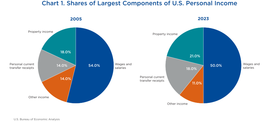
Chart 1 shows the shares of the three largest components of personal income for the United States—wage and salary disbursements, property income (dividend income, interest income, and rental income), and personal current transfer receipts—at the beginning and end of our sample period. The share of wages and salaries, the largest component of personal income, has decreased from about 54 percent in 2005 to 50 percent in 2023, while the shares of property income and personal current transfer receipts have increased to 21 and 18 percent, respectively. During the Great Recession and the COVID–19 pandemic, the share of property income temporarily decreased but recovered and grew thereafter. Meanwhile, the share of personal current transfer receipts increased during the Great Recession but then remained more elevated than before and spiked above 20 percent during the pandemic to settle just below 20 percent in 2023.
[View larger chart]
Revision schedule for the state estimates
The quarterly estimates of personal income by state are successively revised to incorporate source data that are more complete, more detailed, and otherwise more appropriate than the data that were previously available, and estimates are released according to a schedule.
The preliminary estimates of quarterly personal income by state are released 3 months after the close of the quarter, and the second estimates 3 months later. In September, during the yearly annual update, the quarterly state estimates of the previous year are tied to the first annual state estimate for that year, incorporating more detailed and more reliable source data than the quarterly estimates. Moreover, during the annual update, the quarterly estimates for the preceding 4 years are revised again to reflect revisions to the annual estimates.
Sources of revisions
The quarterly state estimates of all the income components of personal income are based on the growth rates of quarterly state source data or indicator series that are controlled to the U.S. quarterly estimates of personal income and its components published in the BEA National Income and Product Accounts (NIPAs).4
The quarterly state estimates are prepared in five parts: (1) wage and salary disbursements, (2) components based on wages and salaries, (3) farm proprietors' income, (4) Medicaid benefits and unemployment insurance benefits, and (5) components based on annual trends. A summary of the major sources of state data for the preliminary, second, and annual update of quarterly estimates are presented in appendix table N.
Wage and salary disbursements
The preliminary national estimates of wages and salaries are based on a sample of employment from the Current Employment Statistics (CES) program of the U.S. Bureau of Labor Statistics (BLS).5 The national estimates include information on hours worked and average hourly earnings from the CES that are not available for states. Thus, the state estimates of wages and salaries are based only on CES employment by industry by state.
Additionally, the limited CES information consists of only production and non-supervisory workers, and the hourly earnings do not include lump sum payments, such as exercised stock options, stock grants, or other bonus compensation. Also, because the CES is a survey, the information is subject to sampling errors. Therefore, because of the use of less comprehensive source data, the preliminary estimates of wages and salaries are subject to more revision than the second estimates.
The second estimates of wages and salaries are published 3 months after the preliminary estimates, incorporating state-level tabulations of wages from the Quarterly Census of Employment and Wages (QCEW) from BLS. The QCEW covers about 95 percent of total wages disbursed and is therefore considered a near-complete census of wages.6 Annual estimates for wages and salaries are based primarily on QCEW data with additional supplementary annual data for industries where QCEW data does not provide full coverage (appendix table N).
Components based on wages and salaries
The estimates of wages and salaries are used to produce the preliminary quarterly state estimates of employer contributions for employee pensions and insurance funds, proprietors' income for the construction industry, all contributions for government social insurance, and residence adjustment.7 Subsequently, revisions to the second quarterly estimates of these components reflect the revisions to the estimates of wages and salaries as well. Annual estimates for these components are based on annual source data from a variety of federal agencies and other sources (appendix table N).
Farm proprietors' income
Although farm proprietors' income is small nationally, 0.3 percent of personal income in 2023, it is significant in several states, such as North and South Dakota, Nebraska, Kansas, and Idaho, where it accounts for a higher share and for much of the variability of personal income. Moreover, revisions to this income component can be large, given the quickly changing natural and economic conditions affecting the farm sector.
The quarterly state estimates of farm proprietors' income are prepared in nine components: grain output, non-grain output, dairy output, poultry output, meat animals' output, government payments, other income, production expenses, and corporate farm income.
Quarterly state shares for farm components are held constant from the most recent annual update. Preliminary quarterly estimates are calculated from the latest fourth quarter of the state quarterly estimates, from the most recent annual update, by extrapolating using the level changes in the U.S. quarterly estimates for the nine farm components from the NIPAs.
Three months later, the second estimates include revised level changes from the NIPAs that incorporate updated price and quantity information on commodities from the latest U.S. annual farm income forecast from the U.S. Department of Agriculture (USDA). Subsequently, every September, annual estimates for farm proprietors' income incorporate complete annual state-level data from the USDA farm income accounts (appendix table N).
Medicaid benefits and unemployment insurance benefits
Medicaid benefits and unemployment insurance benefits are personal income components within personal current transfer receipts. Both benefit payments are estimated separately from the rest of personal current transfer receipts because quarterly state data is available for each. The quarterly estimates for Medicaid and unemployment insurance benefits are extrapolated from the latest fourth quarter of the state quarterly estimates from the most recent annual update. Preliminary quarterly state estimates of Medicaid benefits are extrapolated and controlled to U.S. estimates from the NIPAs using quarterly state information from the Center for Medicare & Medicaid Services (CMS), CMS–64 Quarterly Expense Report. Preliminary quarterly state estimates of unemployment insurance benefits are extrapolated and controlled to U.S. estimates from the NIPAs using monthly state unemployment rates from BLS. Preliminary quarterly estimates are revised 3 months later during the second estimates to incorporate revised data from the CMS–64 Quarterly Expense Report, revised monthly state unemployment rates from BLS, and revised NIPA estimates. Annual estimates for both types of benefit payments incorporate the latest and most complete state-level data from CMS and BLS. The rest of the components of personal current transfer receipts are estimated quarterly based on annual trends (see the section below for more information). Annual estimates for personal current transfer receipts incorporate complete annual state-level data from a variety of agencies and other sources (appendix table N).
Components based on annual trends
Quarterly state indicators for the following components of state personal income are unavailable: personal dividend income, personal interest income, rental income of persons, personal current transfer receipts excluding Medicaid and unemployment benefits, and proprietors' income excluding construction and farm proprietors' income. The preliminary quarterly state estimates for these income components are based on state shares from the most recent annual estimates from the most recent annual update. U.S. quarterly estimates from the NIPAs are allocated to states based on detailed state share information for each income component to produce quarterly state estimates. Preliminary estimates are subject to revisions primarily due to the incorporation of updated NIPA quarterly estimates. Annual estimates for all these personal income components incorporate complete annual state-level data from a variety of agencies and other sources (appendix table N).
Gross domestic product
GDP measures the market value of the goods and services produced by the economy of an area in a particular period. Also known as value added, GDP is the value of goods and services produced by private industry and government, less the value of goods and services used up in production. GDP can be measured in three different ways. First, GDP can be measured as the sum of expenditures, or purchases, by final users.
+ (Exports − Imports)
Second, because the market price of a good or service will reflect all of the incomes earned and costs incurred in production, GDP can also be measured as the sum of all incomes earned during production. That is, the income earned by the three factors of production: labor, capital, and government.8
+ Taxes on production and imports − Subsidies
Third, GDP can also be measured either as total sales less the value of intermediate inputs; or as the sum of the value added at each stage of the production process. The “value added” approach is central to BEA's GDP by industry estimates.
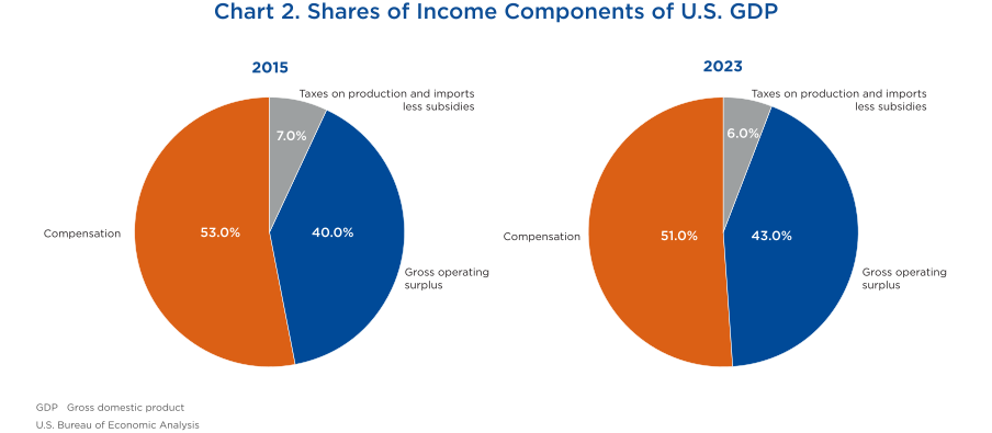
BEA measures GDP by state using the second, or income-earned, approach because of the availability of state level data to do so. The income composition of GDP has shifted slightly from 2015 to 2023. Compensation earned by employees has decreased from 53 percent to 51 percent, while gross operating surplus, the income earned by capital, has grown from 40 percent to 43 percent, as shown in chart 2.
[View larger chart]
Revision schedule for the state estimates
BEA has been producing official quarterly estimates of GDP by state since December 2015 with the release of estimates for the second quarter of 2015. The preliminary estimates of quarterly GDP by state are now released 3 months after the close of the quarter along with the personal income by state estimates. The preliminary quarterly estimates of GDP by state are revised only annually during the annual update, released in September, to incorporate annual source data that are more complete, more detailed, and otherwise more appropriate than the data that were initially available. During the annual update, the quarterly estimates for the preceding 4 years are revised to reflect revisions to the annual GDP by state estimates.
Sources of revisions
The quarterly state estimates are based on the growth rates of quarterly state source data that are controlled to BEA's national quarterly GDP by industry estimates. The GDP by state estimates are scaled to the national GDP estimates minus overseas activity.9 The quarterly state estimates are prepared in two parts: (1) current-dollar GDP by state estimates, and (2) real, or inflation-adjusted, GDP by state estimates. A summary of the major sources of state data for the preliminary and annual update of quarterly estimates are presented in appendix table O.
Current-dollar GDP by state
The methodology used to produce the quarterly GDP by state estimates relies heavily on annual estimates of GDP by state, quarterly estimates of national GDP by industry, and quarterly estimates of personal income by state. Quarterly earnings by industry at the state level are used to extrapolate quarterly GDP by state and industry values from the latest fourth quarter of the state quarterly estimates from the most recent annual update.10 These initial quarterly GDP by state estimates are then scaled to the quarterly national GDP by industry estimates. In contrast, the annual estimates of GDP by state are estimated by income component—compensation of employees, gross operating surplus, taxes on production and imports, and subsidies—and industry separately. The annual estimates of GDP by state incorporate annual state-level data from a variety of agencies and other sources (appendix table O).
Real GDP by state
Estimates of real GDP by state and industry are created by directly deflating the current-dollar estimates for detailed industries using national chain-type price indexes. Real estimates are then calculated for the four aggregate industries—all industries, private industries, manufacturing, and government—using the same chain-type index formula used in the national accounts.11 This method directly correlates to the deflation process used for detailed industries for the annual state estimates done during the annual update.
There are many different ways of measuring the size and quality of the revisions to estimates. By convention, for every state i, revisions are defined as the later vintage estimates less the earlier vintage estimates; that is, for any time t, a revision is
where Lti is the growth rate of the relevant economic state variable at period t implied by the later vintage estimates, and Eti is corresponding growth rate implied by the earlier vintage estimates. For total personal income and its components, revisions to quarterly growth rates are shown to make them easily comparable to von Kerczek and Lopez (2012).12 For GDP by state, revisions to annualized quarterly growth rates are shown to make the analysis consistent with the triennial revisions studies for national GDP.13 The revision study focuses on the four measures of revisions listed below:
- Mean absolute revisions (MARs)
- MARs as a fraction of average growth rate
- Percentage of upward and downward revisions
- Percentage of sign switches in growth between revisions
Mean revisions and mean absolute revisions
The mean revision for state i (MRi) is the average of the revisions in the sample period.

However, since these revisions may be positive one quarter and negative the next, they may offset each other, so mean revisions are not informative on their own. A more useful way to measure the quality of revisions is to look at the mean absolute revision for each state i. The mean absolute revision gives us the average size of revisions independent of the sign.

Additionally, to assess our revisions, the underlying average growth rate in the sample period for a state is also important. For example, think of state A with an average growth rate of 4 percent across the sample period and state B with an average growth rate of 1 percent. Imagine that for both states, A and B, in one quarter the initial estimates of growth are 1 percent and in the subsequent vintage of estimates it is 1.5 percent. With growth in state A on average at 4 percent and in state B at 1 percent, the estimates for state A are more reliable than for state B as the revision of 1/2 percentage point is a much smaller fraction of 4 percent than 1 percent. Thus, to account for this, the revision study includes both analysis of the mean absolute revision of growth and the mean absolute revision as a fraction of the average growth. The analysis is done for all states and the District of Columbia on total personal income, major components of personal income, and GDP.
Similarly, in order to account for the difficulty of estimating a series ex-ante, it is important not only to look at the average growth of the underlying series, but also to its standard deviation, as volatile series are harder to estimate, and are much more likely to have larger revisions.
For that purpose, it is also useful to calculate the coefficient of variation (CVi), which is the standard deviation of a series divided by its average.

Average quarterly growth and volatility
As discussed above, the three largest components of personal income are wage and salary disbursements, property income (dividend income, interest income, and rental income), and personal current transfer receipts. It is worth reiterating that chart 1 showed how the share of wages and salaries, the largest component of personal income, has decreased from 54 percent in 2005 to 50 percent in 2023, while the shares of property income and personal current transfer receipts have increased.
Another way to look at how these shares have evolved over time is to compare the average quarterly growth of each major personal income component, measured by our latest estimates, to the average growth of personal income in our sample period. See appendix table A.
The bottom line of appendix table A shows that for all the states, total personal income (TPI) as measured by the latest estimates grew quarterly at an average of 1.1 percent, while wages and salaries (WS) grew slightly less at 1 percent, thus shrinking its share. Property income (DIRR) grew on average 1.3 percent, and personal current transfer receipts (PCT) 2 percent, both increasing their shares of total personal income. These summary statistics point to a possible increase in the difficulty of producing reliable personal income estimates, as the importance of the components for which we have less-timely source data grew.
Appendix table A also shows the volatility of the quarterly growth rates via the standard deviation. The standard deviation for wages and salaries across all states was 1.6 percent, while for property income and personal current transfer receipts it was 2.7 and 12.1 percent, respectively. That is, growth in both property income and personal current transfer receipts is more volatile than growth in wages and salaries. Keep in mind the sample period includes the Great Recession and the COVID–19 pandemic, two periods when the federal government expanded social safety net programs, which temporarily increased personal current transfer receipts.
Results: mean absolute revisions
Table 1 below presents a summary of mean absolute revisions across vintages for personal income and across states from 2005 to 2023. The table shows average mean absolute revision in quarterly growth rates between the preliminary estimates, the second estimates, the first annual estimates, and the latest estimates. The diagonal of the table shows the average mean absolute revision in growth rates between subsequent vintages of personal income.
| Vintage | Average | ||
|---|---|---|---|
| Second | First annual | Latest | |
| Preliminary | 0.57 | 0.63 | 0.78 |
| Second | n.a. | 0.45 | 0.71 |
| First annual | n.a. | n.a. | 0.61 |
U.S. Bureau of Economic Analysis
The average mean absolute revision for personal income across all states from one estimate to the next is similar in size, 0.57 between the preliminary and second estimates, 0.45 between the second and first annual estimates, and 0.61 between the first annual and latest estimates. This is primarily because the timing of new data being incorporated into the main components of personal income is evenly spaced between estimate vintages. Also important, notice the average mean absolute revision between the preliminary and latest estimates is smaller than the sum of the three vintage-to-vintage mean absolute revisions of the diagonal elements. This indicates that new data and estimates are not independent of previous ones, but build and interconnect with each other.
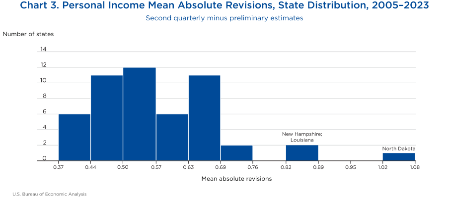
Chart 3 shows the state distribution of the mean absolute revision between the preliminary and second estimates. For most states, the mean absolute revision between the two vintages of estimates is close to the overall average of 0.57. Only a few states like North Dakota, New Hampshire, or Louisiana show significantly larger revisions. To see each state's mean absolute revision vintage to vintage, see appendix table B.
[View larger chart]
To better understand the reasons behind the revisions to the state personal income estimates, it is useful to look at the same mean absolute revision analysis for the three largest income components of personal income.
Table 2 shows the average mean absolute revision in quarterly growth rates across states between the different vintages of wages and salaries from 2005 to 2023. Analogous to the personal income table, the diagonal of table 2 shows the average mean absolute revision in quarterly growth rates between the different vintages of wages and salaries.
| Vintage | Average | ||
|---|---|---|---|
| Second | First annual | Latest | |
| Preliminary | 0.95 | 0.86 | 0.87 |
| Second | n.a. | 0.49 | 0.60 |
| First annual | n.a. | n.a. | 0.48 |
- n.a.
- Not applicable
U.S. Bureau of Economic Analysis
Here, consistent with the incorporation of source data explained above, the largest revision of 0.95 occurs between the preliminary and the second quarterly estimate when the CES data is substituted with the more comprehensive QCEW data into the estimates of wages and salaries. The revisions between the second quarterly and the first annual estimates, and between the first annual and the latest estimates, are half in size, 0.49 and 0.48 respectively.
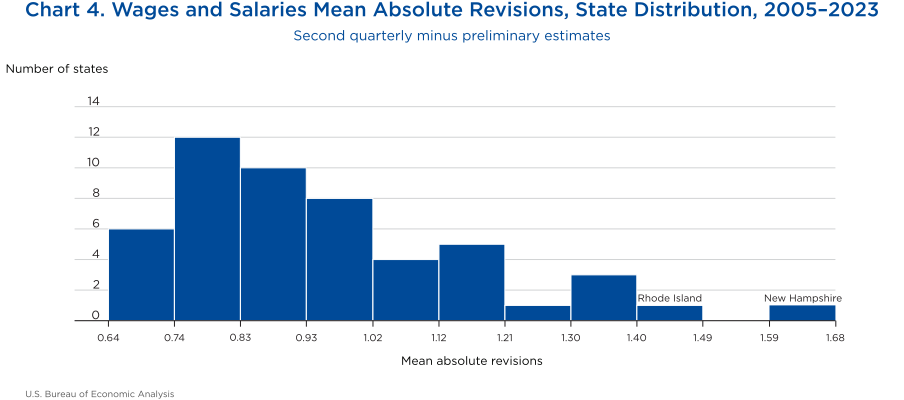
Chart 4 shows the state distribution of mean absolute revision between the preliminary and second quarterly estimates. In 30 states and the District of Columbia, the mean absolute revision between the two vintages of estimates is less than the overall average of 0.95, while 15 states are just above the average, between 1.0 and 1.2. New Hampshire shows the largest mean absolute revisions. The large revisions to wages and salaries in New Hampshire are due to differences between estimates based on CES data (preliminary estimates) and estimates based on QCEW data (second quarterly estimates). To see each state's mean absolute revision for wages and salaries between vintages, see appendix table C.
[View larger chart]
Table 3 shows the average mean absolute revision in quarterly growth rates across states between the different vintages of property income from 2005 to 2023. Again, the diagonal of the table shows the average mean absolute revision between each successive vintage. Since the best and most complete source data for the property income estimates are annual data from the Internal Revenue Service that are available with a two-year lag, the diagonal shows that the largest revision happens after the first annual update has taken place, 1.74. Moreover, the table also shows that the revisions to property income can be large, so it can be expected that states with higher than average shares of personal income generated by property income can have relatively larger mean absolute revisions to total personal income, too.
| Vintage | Average | ||
|---|---|---|---|
| Second | First annual | Latest | |
| Preliminary | 0.32 | 1.04 | 1.85 |
| Second | n.a. | 0.95 | 1.94 |
| First annual | n.a. | n.a. | 1.74 |
- n.a.
- Not applicable
U.S. Bureau of Economic Analysis
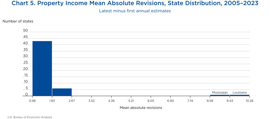
Chart 5 shows the state distribution of the mean absolute revision between the first annual and the latest estimates. Forty-eight states and the District of Columbia are close to the average of 1.74. Only Louisiana and Mississippi have much larger revisions. Estimates of property income in 2005 and 2006 were significantly impacted by hurricane Katrina, causing the mean absolute revision for both states to be bigger than typically expected. To see each state's mean absolute revision for property income between vintages, see appendix table D.
[View larger chart]
Table 4 shows the average mean absolute revision across states in quarterly growth rates between the different vintages of personal current transfer receipts from 2005 to 2023. The table shows that better and more complete source data used to compute the estimates of personal current transfers receipts are introduced during each vintage, with revisions between the second quarterly and the first annual estimates at 0.83, and between the first annual and the latest estimates at 1.00.
| Vintage | Average | ||
|---|---|---|---|
| Second | First annual | Latest | |
| Preliminary | 0.43 | 0.94 | 1.40 |
| Second | n.a. | 0.83 | 1.32 |
| First annual | n.a. | n.a. | 1.00 |
- n.a.
- Not applicable
U.S. Bureau of Economic Analysis
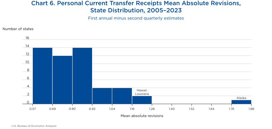
Chart 6 shows the state distribution of the mean absolute revision between the second quarterly and the first annual estimates. The largest revisions occur in Alaska, where information on the amount of the annual payment to individuals from the Alaska Permanent Fund Dividend is not available until the first annual estimates. To see each state's mean absolute revision for personal current transfer receipts between vintages, see appendix table E.
[View larger chart]
Industry composition, growth, and volatility
Between 2015, the first year in which BEA began officially releasing quarterly GDP by state statistics, and the end of 2023, the national shares of income generated by labor (compensation) and capital (gross operating surplus) during the production of GDP shifted away from labor and towards capital. Chart 2 above shows compensation shrank 2 percent from 53 percent to 51 percent while gross operating surplus increased 3 percent from 40 percent to 43 percent. The shares of these two income components to GDP vary greatly by state and by industry. States with economies that have a diverse mix of industries tend to exhibit a similar GDP share of compensation and gross operating surplus as the United States. States whose economies have a high relative concentration of industries more reliant on capital, such as agriculture and mining, tend to exhibit a greater GDP share of gross operating surplus relative to compensation.
Appendix table F shows basic statistics—the mean growth rate, the standard deviation, and the coefficient of variation—by state of annualized quarterly real GDP growth for BEA's latest estimates. Small states, those with small populations or small in geographic size, like Wyoming, North Dakota, Alaska, and Delaware, have the biggest coefficients of variation indicating these states are the most susceptible to bigger revisions across the vintages of quarterly GDP estimates. These states exhibit small mean growth rates across 2015 to 2023 with large standard deviations resulting in large coefficients of variation.
A large coefficient of variation may also indicate states whose economies have a less diversified industrial base, making their GDP estimates more sensitive to estimates for a particular industry. The states in appendix table F are ordered from lowest to highest by coefficient of variation, ranging from Utah (the lowest coefficient of variation) to Wyoming (the highest).
Results: mean absolute revisions
Table 5 presents the average mean absolute revision across states in annualized quarterly growth rates for GDP between the preliminary, first annual, and latest estimates from 2015 to 2023. The diagonal figures in the table show the revision from one vintage to the next.
| Vintage | First annual | Latest |
|---|---|---|
| Average | ||
| Preliminary | 2.29 | 2.64 |
| First annual | n.a. | 1.99 |
| Weighted average | ||
| Preliminary | 1.98 | 2.26 |
| First annual | n.a. | 1.71 |
| Median | ||
| Preliminary | 2.16 | 2.42 |
| First annual | n.a. | 1.75 |
- GDP
- Gross domestic product
- n.a.
- Not applicable
U.S. Bureau of Economic Analysis
The top of the table shows the unweighted average among all states. The revision between the preliminary and first annual estimates is 2.29 percent, while the revision between the preliminary and the latest estimates is 2.64 percent. The revision between the first annual and the latest estimates is 1.99 percent. The small difference between the revision between the preliminary and first annual estimates and the revision between the preliminary and the latest estimates indicates the revisions are related more to a reallocation of growth among states as opposed to a revision in average level of growth.
The middle of the table shows the mean absolute revision for the median state. The bottom of the table shows the mean absolute revision for the weighted average across all states and the District of Columbia using 2023 real GDP levels for the weights. The results show the mean absolute revision getting smaller across all instances as you move from the median to the weighted average.
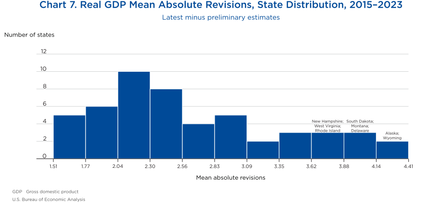
Chart 7 shows the state distribution of mean absolute revision between the preliminary and the latest estimates. Twenty-nine states have a mean absolute revision less than the overall average of 2.64 percent. States that are less populated and less industry-diversified like Alaska, Wyoming, Montana, South Dakota, and Delaware have larger than average mean absolute revisions. To see each state's mean absolute revision between vintages see appendix table G.
[View larger chart]
Revisions to annualized quarterly growth rates for the state real GDP estimates can also be assessed by taking into account the size of the mean absolute revision between vintages relative to the growth rate of the latest estimate. This is done by dividing the mean absolute revision for each state by the average annualized quarterly growth rate for the latest estimates. Results are shown in table 6.
| Latest | Absolute (latest−first annual)/latest | Absolute (latest−preliminary)/latest |
|---|---|---|
| United States | 0.3 | 0.3 |
| Florida | 0.3 | 0.4 |
| Utah | 0.4 | 0.5 |
| Tennessee | 0.5 | 0.5 |
| Washington | 0.4 | 0.6 |
| Arizona | 0.4 | 0.6 |
| North Carolina | 0.6 | 0.6 |
| California | 0.5 | 0.6 |
| Colorado | 0.6 | 0.6 |
| Virginia | 0.5 | 0.6 |
| Georgia | 0.6 | 0.6 |
| Nevada | 0.5 | 0.7 |
| New Jersey | 0.7 | 0.7 |
| South Carolina | 0.5 | 0.7 |
| Texas | 0.6 | 0.7 |
| Alabama | 0.5 | 0.7 |
| Idaho | 0.5 | 0.7 |
| Indiana | 0.6 | 0.8 |
| Oregon | 0.5 | 0.8 |
| Massachusetts | 0.6 | 0.8 |
| Ohio | 0.8 | 0.9 |
| New Mexico | 0.9 | 0.9 |
| Maine | 0.6 | 0.9 |
| Kentucky | 0.7 | 0.9 |
| Arkansas | 1.0 | 1.1 |
| Pennsylvania | 1.1 | 1.2 |
| Missouri | 0.8 | 1.2 |
| Vermont | 0.9 | 1.2 |
| Maryland | 1.1 | 1.2 |
| Michigan | 0.8 | 1.2 |
| Minnesota | 1.0 | 1.3 |
| Nebraska | 0.9 | 1.3 |
| New Hampshire | 0.8 | 1.3 |
| Mississippi | 1.1 | 1.4 |
| Wisconsin | 1.0 | 1.4 |
| New York | 0.9 | 1.4 |
| Montana | 1.1 | 1.5 |
| District of Columbia | 1.3 | 1.5 |
| Illinois | 1.2 | 1.5 |
| Kansas | 1.5 | 1.6 |
| Hawaii | 1.1 | 2.0 |
| South Dakota | 1.9 | 2.0 |
| Rhode Island | 1.2 | 2.2 |
| Oklahoma | 2.0 | 2.2 |
| Connecticut | 2.4 | 2.6 |
| West Virginia | 2.2 | 2.6 |
| Iowa | 2.4 | 2.6 |
| Louisiana | 1.9 | 2.7 |
| North Dakota | 5.2 | 6.3 |
| Delaware | 6.5 | 6.3 |
| Alaska | 4.1 | 6.4 |
| Wyoming | 11.3 | 14.0 |
- GDP
- Gross domestic product
U.S. Bureau of Economic Analysis
The United States is at the top of the table with the states sorted below by the far-right column—the ratio of the mean absolute revision from the preliminary to latest estimates divided by the average annualized quarterly growth rate from the latest estimates—from the smallest to the largest. States that are less populated and less industry diversified are at the bottom, while big and industry-diversified states are at the top.
Comparing Florida and Utah, states at the top of the table, with Wyoming and Alaska, states at the bottom of the table, provides interesting context for understanding revisions to state GDP growth rates. Florida and Utah are more populated and industry diversified. In contrast, Wyoming and Alaska are states with comparatively smaller populations and economies with less diverse industry mix, as they are reliant on specific industries. In 2023, total population in Florida and Utah was 22.9 and 3.4 million, respectively, while total population in Wyoming and Alaska was 584,666 and 734,654, respectively. Additionally in 2023, Florida had only one industry with an industry specialization index above 5, and Utah had none. Meanwhile, Alaska had five industries with a specialization index above 5—led by pipeline transportation and mining (except oil and gas)— and Wyoming had six industries—led by mining (except oil and gas), rail transportation, and pipeline transportation.14
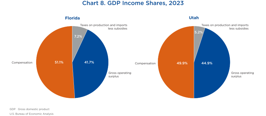
The income composition of a state's GDP can play an important role in the magnitude of revisions to that state's GDP estimates. Chart 8 shows the income component shares of GDP for Florida and Utah. In both states' compensation, the income generated by labor is 50 percent or more. Both states have economies with a diverse industry mix, GDP more reliant on labor income, and smaller revisions.
[View larger chart]
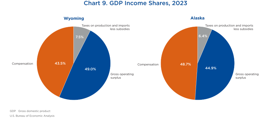
The picture in Wyoming and Alaska is different. Chart 9 shows gross operating surplus in Wyoming is larger than compensation, while, in Alaska, gross operating surplus is nearly the same size as compensation. Wyoming and Alaska have economies with a less diverse industry mix, reliant on specific capital-intensive industries, with GDP more reliant on income generated by capital, and larger revisions.
[View larger chart]
The quarterly state source data, industry earnings by state, used to prepare the preliminary estimates of GDP by state are a good indicator of growth for the labor portion of GDP, compensation, but less effective as an indicator of growth for the capital portion of GDP, gross operating surplus. Better source data to measure gross operating surplus is not incorporated until the first annual and latest estimates.
Because revisions are repeated estimations of the economic activity in a period, their patterns, and not only their size, provide a measure of the reliability of the estimates. The next section examines the qualitative characteristics of the quarterly state estimates of personal income and GDP across vintages.
The patterns of quarterly growth, including whether growth in any period is high or low relative to trend, is accelerating or decelerating, or is positive or negative, are key to understanding the pulse of economic growth at the regional level. In this section, the direction of revisions to growth as well as the sign of growth in different vintages of personal income and real GDP are examined.
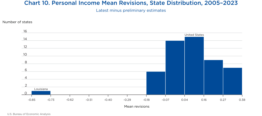
Upward and downward revisions to growth are, on average, expected to cancel each other if there is no estimation bias across estimate vintages. Chart 10 shows the distribution of mean revisions by state between the latest and the preliminary estimates of quarterly personal income growth. See appendix table H for detailed results.
As expected, an overwhelming majority of states have small mean revisions close to 0, indicating no bias across estimate vintages. Idaho, Utah, Wyoming, and Montana have positive mean revisions of personal income over 0.30 percentage points, while Louisiana has an average negative mean revision of −0.85 percentage points, due to the impacts of Hurricane Katrina.
[View larger chart]
Appendix table I shows the percentage of upward revisions between the preliminary and the latest personal income estimates for each state between 2005 and 2023. Latest estimates are revised upward between 40 and 60 percent of the time for most states, also indicating a lack of bias in the revisions across estimate vintages.
Appendix table J shows the patterns of sign switches between the preliminary and latest estimates of quarterly personal income growth by state. At the top of the table are the states with fewer sign switches, led by Tennessee, Florida, Colorado, Arizona, and Washington, while at the bottom are Delaware and North Dakota with the highest percentage of sign switches. Across all states on average, the preliminary and latest estimates display the same sign or direction of growth more than 89 percent of the time. In general, sign switches in growth of personal income across estimate vintages are unusual. The preliminary estimates provide a very reliable picture of current regional economic conditions and their trajectories.
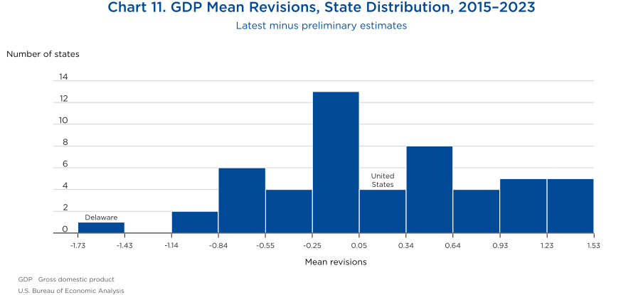
Chart 11 shows the distribution of mean revisions by state between the latest and the preliminary estimates of annualized quarterly real GDP growth. See appendix table K for detailed results.
[View larger chart]
Again, a majority of states have small mean revisions close to 0, between −1 and 1 percentage point, indicating no estimation bias across estimate vintages. Only Idaho and Utah have positive average revisions larger than 1.30 percentage points. Delaware is the only state with a negative average mean revision larger than −1.30 percentage points.
Appendix table L shows the percentage of upward revisions between the preliminary and the latest real GDP growth estimates for each state between 2015 and 2023. For most states, the latest estimates are revised upward between 40 and 60 percent of the time, indicating a lack of bias in the revisions across estimate vintages. However, there are some states, like Florida, Utah, and Washington, whose latest estimates are revised upward more than 66 percent of the time. On the other end, there is Louisiana whose latest estimates are revised downward more than 66 percent of the time.
Appendix table M shows the patterns in percentage terms between the signs of the preliminary and latest estimates of quarterly annualized real GDP growth for each state. At the top of the table are the states with fewer sign switches, led by Florida, where there were none, closely followed by California, Alabama, Arizona, and South Carolina. At the bottom, West Virginia and Delaware show the highest percentage of sign switches, at slightly more than 40 percent of the time. Across all states on average, more than 80 percent of the time the preliminary and latest estimates have the same sign or direction of growth. This means that if the first estimate indicated positive growth, then the latest estimate confirmed it, and vice versa for the less-often cases of negative growth.
In many of the cases where the direction of growth between the preliminary and the latest estimates differed, the sign of growth in the preliminary estimate was slightly positive, and in the latest estimate it turned slightly negative. Occasional changes in direction of growth between vintages is consistent with the difficulty in estimating turning points in the business cycle.
During all periods of the business cycle, including crises such as the COVID–19 pandemic, the private sector and policymakers rely on BEA's state estimates of personal income and GDP to provide a timely, comprehensive, and accurate picture of the economic conditions within the different regions of the United States and inform their economic decisions.
This study has focused on the reliability of the different vintages of both measures through the end of 2023.
As highlighted in the study, U.S. states' populations and economic activity are very heterogeneous in nature, and industries are not spread evenly among states. Thus, since both the industry composition of GDP and the different sources of personal income vary by state, both measures complement each other.
Moreover, because source data do not arrive uniformly over time, BEA releases successive estimates or vintages, each regularly incorporating and aggregating new information in a regular manner. This study examined systematically how those vintages change from one to the next for both state personal income and its major components and state GDP.
More specifically, the results in the study show that the state estimates of quarterly personal income growth and the growth of major income components have relatively small mean absolute revisions from the period between the first quarter of 2005 through the fourth quarter of 2023, results that are consistent with previous, similar BEA studies.15 The results of the study also show that these estimates are reliable, with revisions in subsequent vintages of estimates appearing due to the incorporation of new data and not by systematic measurement biases or errors.
Additionally, the study is the first to analyze the reliability, across estimate vintages, of annualized quarterly growth of state GDP. Analysis of mean absolute revisions, relative mean absolute revisions weighted by growth, and other qualitative measures all indicate the preliminary estimates of state GDP are reliable.
The timeliness and reliability of BEA's state personal income and GDP estimates provide a solid foundation for economic decision-making at both the public and private sector levels.
| State | Total personal income | Wages and salaries | Property income (dividends, interest, rents, and royalties) | Personal current transfer receipts | |||||
|---|---|---|---|---|---|---|---|---|---|
| Mean | Standard deviation | Coefficient of variation | Mean | Standard deviation | Mean | Standard deviation | Mean | Standard deviation | |
| Alabama | 1.0 | 2.5 | 2.4 | 0.9 | 1.4 | 1.1 | 2.2 | 1.9 | 11.1 |
| Alaska | 1.0 | 2.1 | 2.0 | 0.9 | 1.5 | 1.2 | 2.3 | 2.1 | 12.2 |
| Arizona | 1.3 | 2.4 | 1.8 | 1.2 | 1.6 | 1.4 | 2.6 | 2.2 | 11.5 |
| Arkansas | 1.2 | 2.7 | 2.3 | 1.0 | 1.4 | 1.8 | 3.8 | 1.8 | 10.6 |
| California | 1.2 | 1.9 | 1.6 | 1.2 | 1.8 | 1.4 | 2.7 | 2.0 | 11.6 |
| Colorado | 1.4 | 1.9 | 1.4 | 1.3 | 1.6 | 1.7 | 2.8 | 2.5 | 13.1 |
| Connecticut | 0.9 | 1.7 | 1.9 | 0.7 | 1.8 | 1.2 | 2.9 | 1.7 | 11.2 |
| Delaware | 1.0 | 2.4 | 2.4 | 0.8 | 2.0 | 1.2 | 2.4 | 2.1 | 10.0 |
| District of Columbia | 1.2 | 1.6 | 1.3 | 1.0 | 1.2 | 1.3 | 2.9 | 1.9 | 11.4 |
| Florida | 1.3 | 2.2 | 1.7 | 1.2 | 1.8 | 1.5 | 3.1 | 2.0 | 10.6 |
| Georgia | 1.2 | 2.4 | 2.0 | 1.1 | 1.6 | 1.4 | 2.6 | 2.4 | 13.8 |
| Hawaii | 1.0 | 2.2 | 2.1 | 0.9 | 2.0 | 1.2 | 2.2 | 2.3 | 14.3 |
| Idaho | 1.5 | 2.3 | 1.6 | 1.3 | 1.4 | 1.7 | 3.1 | 2.4 | 12.6 |
| Illinois | 0.9 | 1.9 | 2.1 | 0.8 | 1.5 | 1.1 | 2.8 | 1.9 | 12.2 |
| Indiana | 1.1 | 2.2 | 2.0 | 0.9 | 1.7 | 1.1 | 2.4 | 2.0 | 12.0 |
| Iowa | 1.0 | 2.4 | 2.4 | 0.9 | 1.1 | 1.2 | 2.3 | 2.0 | 12.3 |
| Kansas | 1.1 | 2.0 | 1.8 | 0.9 | 1.4 | 1.2 | 2.9 | 1.9 | 12.0 |
| Kentucky | 1.0 | 2.7 | 2.6 | 0.9 | 1.6 | 1.1 | 2.3 | 1.9 | 11.2 |
| Louisiana | 1.0 | 2.8 | 2.7 | 0.8 | 1.5 | 1.3 | 4.3 | 1.9 | 12.2 |
| Maine | 1.0 | 2.4 | 2.3 | 0.9 | 1.6 | 1.2 | 2.1 | 1.8 | 11.1 |
| Maryland | 0.9 | 1.8 | 1.9 | 0.9 | 1.3 | 1.0 | 2.0 | 2.1 | 12.1 |
| Massachusetts | 1.1 | 1.7 | 1.5 | 1.0 | 1.7 | 1.5 | 2.9 | 2.0 | 13.6 |
| Michigan | 0.9 | 2.7 | 3.1 | 0.7 | 2.3 | 1.1 | 2.8 | 2.0 | 14.3 |
| Minnesota | 1.1 | 2.1 | 2.0 | 0.9 | 1.6 | 1.3 | 2.7 | 2.1 | 12.9 |
| Mississippi | 1.0 | 3.1 | 3.3 | 0.8 | 1.4 | 1.1 | 3.1 | 1.8 | 12.0 |
| Missouri | 1.0 | 2.2 | 2.1 | 0.9 | 1.6 | 1.3 | 2.9 | 1.9 | 11.4 |
| Montana | 1.4 | 2.4 | 1.8 | 1.2 | 1.3 | 1.6 | 2.6 | 2.2 | 12.6 |
| Nebraska | 1.2 | 2.2 | 1.9 | 1.0 | 1.1 | 1.3 | 2.5 | 2.0 | 12.5 |
| Nevada | 1.3 | 2.5 | 2.0 | 1.1 | 3.1 | 1.5 | 3.1 | 2.7 | 15.4 |
| New Hampshire | 1.0 | 1.6 | 1.6 | 1.0 | 2.4 | 1.3 | 3.0 | 2.0 | 11.9 |
| New Jersey | 1.0 | 1.6 | 1.7 | 0.8 | 1.8 | 1.1 | 2.6 | 1.8 | 11.7 |
| New Mexico | 1.1 | 2.7 | 2.5 | 0.9 | 1.5 | 1.2 | 2.3 | 2.0 | 11.0 |
| New York | 1.0 | 2.1 | 2.1 | 1.0 | 2.5 | 1.3 | 2.8 | 1.6 | 11.9 |
| North Carolina | 1.3 | 2.4 | 1.9 | 1.2 | 1.5 | 1.4 | 2.4 | 2.2 | 11.6 |
| North Dakota | 1.4 | 2.7 | 1.9 | 1.4 | 2.1 | 1.7 | 3.6 | 2.1 | 13.8 |
| Ohio | 0.9 | 2.3 | 2.4 | 0.8 | 1.5 | 1.2 | 2.5 | 1.8 | 12.0 |
| Oklahoma | 1.2 | 2.8 | 2.4 | 1.0 | 1.5 | 1.2 | 2.5 | 2.0 | 11.7 |
| Oregon | 1.3 | 2.1 | 1.6 | 1.1 | 1.5 | 1.5 | 2.7 | 2.1 | 10.6 |
| Pennsylvania | 1.0 | 2.0 | 2.1 | 0.9 | 1.6 | 1.2 | 2.5 | 1.8 | 11.7 |
| Rhode Island | 0.9 | 2.1 | 2.4 | 0.8 | 2.2 | 0.9 | 2.2 | 1.7 | 12.3 |
| South Carolina | 1.3 | 2.5 | 1.9 | 1.1 | 1.4 | 1.5 | 2.5 | 2.1 | 11.5 |
| South Dakota | 1.3 | 2.4 | 1.8 | 1.2 | 1.2 | 1.5 | 2.7 | 2.2 | 13.0 |
| Tennessee | 1.2 | 2.1 | 1.8 | 1.1 | 1.6 | 1.4 | 2.2 | 1.9 | 11.6 |
| Texas | 1.4 | 2.3 | 1.6 | 1.3 | 1.5 | 1.7 | 3.0 | 2.3 | 13.2 |
| United States | 1.1 | 2.0 | 1.7 | 1.0 | 1.5 | 1.3 | 2.5 | 2.0 | 11.9 |
| Utah | 1.6 | 2.3 | 1.4 | 1.5 | 1.4 | 1.9 | 3.0 | 2.7 | 15.2 |
| Vermont | 1.0 | 2.3 | 2.4 | 0.9 | 1.6 | 1.1 | 2.9 | 2.0 | 12.8 |
| Virginia | 1.1 | 1.8 | 1.7 | 1.0 | 1.2 | 1.2 | 2.3 | 2.2 | 11.6 |
| Washington | 1.3 | 2.2 | 1.7 | 1.4 | 1.4 | 1.2 | 5.2 | 2.2 | 12.9 |
| West Virginia | 1.0 | 3.0 | 3.1 | 0.8 | 1.6 | 1.0 | 2.0 | 1.6 | 10.5 |
| Wisconsin | 1.0 | 2.0 | 2.0 | 0.9 | 1.4 | 1.2 | 2.6 | 1.9 | 11.3 |
| Wyoming | 1.3 | 2.5 | 1.9 | 1.0 | 2.1 | 1.6 | 4.0 | 2.1 | 12.0 |
U.S. Bureau of Economic Analysis
| State | Estimates | |||
|---|---|---|---|---|
| Second−preliminary | First annual−second | Latest−first annual | Latest−preliminary | |
| Alabama | 0.37 | 0.33 | 0.32 | 0.46 |
| Alaska | 0.67 | 0.52 | 0.51 | 0.82 |
| Arizona | 0.55 | 0.42 | 0.54 | 0.62 |
| Arkansas | 0.63 | 0.54 | 0.56 | 0.82 |
| California | 0.59 | 0.39 | 0.40 | 0.73 |
| Colorado | 0.53 | 0.38 | 0.58 | 0.86 |
| Connecticut | 0.66 | 0.42 | 0.64 | 0.65 |
| Delaware | 0.70 | 0.53 | 0.75 | 0.86 |
| District of Columbia | 0.52 | 0.49 | 0.75 | 0.74 |
| Florida | 0.42 | 0.38 | 0.59 | 0.72 |
| Georgia | 0.44 | 0.32 | 0.46 | 0.68 |
| Hawaii | 0.51 | 0.36 | 0.56 | 0.66 |
| Idaho | 0.61 | 0.52 | 0.65 | 0.84 |
| Illinois | 0.51 | 0.41 | 0.39 | 0.61 |
| Indiana | 0.49 | 0.33 | 0.49 | 0.54 |
| Iowa | 0.64 | 0.67 | 0.67 | 0.87 |
| Kansas | 0.58 | 0.53 | 0.71 | 0.89 |
| Kentucky | 0.48 | 0.41 | 0.46 | 0.62 |
| Louisiana | 0.86 | 0.62 | 2.70 | 2.41 |
| Maine | 0.56 | 0.35 | 0.48 | 0.62 |
| Maryland | 0.39 | 0.31 | 0.41 | 0.45 |
| Massachusetts | 0.66 | 0.38 | 0.48 | 0.71 |
| Michigan | 0.52 | 0.36 | 0.49 | 0.68 |
| Minnesota | 0.57 | 0.41 | 0.50 | 0.65 |
| Mississippi | 0.51 | 0.46 | 0.60 | 0.73 |
| Missouri | 0.48 | 0.28 | 0.47 | 0.58 |
| Montana | 0.55 | 0.53 | 0.61 | 0.73 |
| Nebraska | 0.67 | 0.66 | 0.82 | 0.93 |
| Nevada | 0.69 | 0.57 | 0.68 | 1.00 |
| New Hampshire | 0.86 | 0.43 | 0.57 | 0.89 |
| New Jersey | 0.49 | 0.43 | 0.47 | 0.64 |
| New Mexico | 0.48 | 0.42 | 0.49 | 0.67 |
| New York | 0.65 | 0.51 | 0.62 | 0.76 |
| North Carolina | 0.48 | 0.38 | 0.62 | 0.77 |
| North Dakota | 1.08 | 1.24 | 0.90 | 1.45 |
| Ohio | 0.42 | 0.30 | 0.39 | 0.51 |
| Oklahoma | 0.53 | 0.55 | 0.96 | 1.12 |
| Oregon | 0.50 | 0.37 | 0.48 | 0.67 |
| Pennsylvania | 0.47 | 0.29 | 0.48 | 0.57 |
| Rhode Island | 0.74 | 0.43 | 0.57 | 0.85 |
| South Carolina | 0.38 | 0.31 | 0.45 | 0.58 |
| South Dakota | 0.68 | 1.03 | 0.88 | 1.03 |
| Tennessee | 0.44 | 0.36 | 0.45 | 0.56 |
| Texas | 0.48 | 0.38 | 0.59 | 0.75 |
| United States | 0.37 | 0.25 | 0.37 | 0.48 |
| Utah | 0.65 | 0.49 | 0.69 | 0.84 |
| Vermont | 0.64 | 0.40 | 0.53 | 0.65 |
| Virginia | 0.40 | 0.29 | 0.40 | 0.52 |
| Washington | 0.46 | 0.35 | 0.58 | 0.76 |
| West Virginia | 0.54 | 0.32 | 0.44 | 0.60 |
| Wisconsin | 0.60 | 0.36 | 0.46 | 0.69 |
| Wyoming | 0.67 | 0.64 | 0.87 | 1.20 |
U.S. Bureau of Economic Analysis
| State | Estimates | |||
|---|---|---|---|---|
| Second−preliminary | First annual−second | Latest−first annual | Latest−preliminary | |
| Alabama | 0.64 | 0.37 | 0.37 | 0.67 |
| Alaska | 1.11 | 0.61 | 0.44 | 0.93 |
| Arizona | 0.96 | 0.48 | 0.56 | 0.84 |
| Arkansas | 1.08 | 0.72 | 0.53 | 1.01 |
| California | 1.04 | 0.40 | 0.40 | 0.99 |
| Colorado | 0.87 | 0.43 | 0.45 | 0.82 |
| Connecticut | 1.27 | 0.58 | 0.62 | 1.05 |
| Delaware | 1.36 | 0.71 | 0.77 | 1.13 |
| District of Columbia | 0.88 | 0.41 | 0.43 | 0.73 |
| Florida | 0.86 | 0.43 | 0.42 | 0.82 |
| Georgia | 0.70 | 0.32 | 0.38 | 0.66 |
| Hawaii | 0.90 | 0.58 | 0.61 | 0.72 |
| Idaho | 0.96 | 0.62 | 0.46 | 0.87 |
| Illinois | 0.81 | 0.40 | 0.40 | 0.74 |
| Indiana | 0.85 | 0.36 | 0.46 | 0.78 |
| Iowa | 0.86 | 0.43 | 0.48 | 0.76 |
| Kansas | 0.98 | 0.46 | 0.51 | 0.90 |
| Kentucky | 0.82 | 0.39 | 0.40 | 0.78 |
| Louisiana | 0.97 | 0.51 | 0.48 | 0.87 |
| Maine | 1.02 | 0.43 | 0.49 | 0.92 |
| Maryland | 0.79 | 0.43 | 0.44 | 0.75 |
| Massachusetts | 1.12 | 0.54 | 0.50 | 0.94 |
| Michigan | 0.93 | 0.49 | 0.57 | 0.96 |
| Minnesota | 0.94 | 0.51 | 0.49 | 0.90 |
| Mississippi | 0.78 | 0.36 | 0.38 | 0.77 |
| Missouri | 0.83 | 0.41 | 0.43 | 0.78 |
| Montana | 0.87 | 0.60 | 0.47 | 0.73 |
| Nebraska | 0.87 | 0.48 | 0.41 | 0.72 |
| Nevada | 1.34 | 0.54 | 0.60 | 1.27 |
| New Hampshire | 1.68 | 0.56 | 0.54 | 1.44 |
| New Jersey | 0.71 | 0.47 | 0.52 | 0.73 |
| New Mexico | 0.81 | 0.42 | 0.49 | 0.71 |
| New York | 1.31 | 0.63 | 0.67 | 1.33 |
| North Carolina | 0.79 | 0.39 | 0.36 | 0.77 |
| North Dakota | 1.18 | 0.62 | 0.48 | 0.99 |
| Ohio | 0.73 | 0.36 | 0.42 | 0.75 |
| Oklahoma | 0.88 | 0.50 | 0.50 | 0.79 |
| Oregon | 0.91 | 0.45 | 0.45 | 0.80 |
| Pennsylvania | 0.78 | 0.35 | 0.47 | 0.82 |
| Rhode Island | 1.45 | 0.63 | 0.59 | 1.31 |
| South Carolina | 0.71 | 0.42 | 0.38 | 0.64 |
| South Dakota | 0.76 | 0.59 | 0.50 | 0.71 |
| Tennessee | 0.83 | 0.48 | 0.43 | 0.76 |
| Texas | 0.75 | 0.41 | 0.39 | 0.72 |
| United States | 0.71 | 0.26 | 0.31 | 0.70 |
| Utah | 0.96 | 0.61 | 0.49 | 0.88 |
| Vermont | 1.15 | 0.51 | 0.53 | 0.81 |
| Virginia | 0.66 | 0.32 | 0.38 | 0.72 |
| Washington | 0.81 | 0.52 | 0.60 | 0.90 |
| West Virginia | 1.13 | 0.55 | 0.56 | 0.90 |
| Wisconsin | 0.98 | 0.43 | 0.48 | 0.95 |
| Wyoming | 1.20 | 0.59 | 0.47 | 1.15 |
U.S. Bureau of Economic Analysis
| State | Estimates | |||
|---|---|---|---|---|
| Second−preliminary | First annual−second | Latest−first annual | Latest−preliminary | |
| Alabama | 0.30 | 0.79 | 1.40 | 1.41 |
| Alaska | 0.30 | 0.86 | 1.20 | 1.28 |
| Arizona | 0.30 | 0.82 | 1.34 | 1.44 |
| Arkansas | 0.32 | 0.95 | 2.12 | 2.14 |
| California | 0.29 | 0.73 | 1.30 | 1.40 |
| Colorado | 0.29 | 0.85 | 1.46 | 1.49 |
| Connecticut | 0.29 | 0.82 | 1.35 | 1.47 |
| Delaware | 0.26 | 0.69 | 1.19 | 1.35 |
| District of Columbia | 0.26 | 0.88 | 1.62 | 1.59 |
| Florida | 0.29 | 0.83 | 1.53 | 1.71 |
| Georgia | 0.25 | 0.74 | 1.29 | 1.42 |
| Hawaii | 0.28 | 0.62 | 1.31 | 1.39 |
| Idaho | 0.28 | 0.90 | 1.69 | 1.80 |
| Illinois | 0.26 | 0.75 | 1.17 | 1.32 |
| Indiana | 0.23 | 0.71 | 0.98 | 1.15 |
| Iowa | 0.21 | 0.73 | 1.30 | 1.25 |
| Kansas | 0.27 | 0.81 | 1.41 | 1.53 |
| Kentucky | 0.23 | 0.71 | 1.41 | 1.38 |
| Louisiana | 2.73 | 1.83 | 10.28 | 7.80 |
| Maine | 0.21 | 0.72 | 1.04 | 1.16 |
| Maryland | 0.22 | 0.65 | 1.04 | 1.13 |
| Massachusetts | 0.27 | 0.78 | 1.46 | 1.51 |
| Michigan | 0.23 | 0.80 | 1.21 | 1.35 |
| Minnesota | 0.21 | 0.69 | 1.27 | 1.41 |
| Mississippi | 0.96 | 7.06 | 8.73 | 13.64 |
| Missouri | 0.24 | 0.72 | 1.40 | 1.57 |
| Montana | 0.25 | 0.93 | 1.57 | 1.59 |
| Nebraska | 0.25 | 0.79 | 1.29 | 1.37 |
| Nevada | 0.29 | 1.02 | 1.88 | 1.72 |
| New Hampshire | 0.23 | 0.96 | 1.73 | 1.74 |
| New Jersey | 0.23 | 0.78 | 1.28 | 1.28 |
| New Mexico | 0.26 | 0.77 | 1.51 | 1.49 |
| New York | 0.30 | 0.97 | 1.67 | 1.54 |
| North Carolina | 0.26 | 0.82 | 1.16 | 1.24 |
| North Dakota | 0.24 | 0.77 | 2.12 | 2.19 |
| Ohio | 0.24 | 0.72 | 1.07 | 1.30 |
| Oklahoma | 0.27 | 0.77 | 1.24 | 1.38 |
| Oregon | 0.25 | 0.72 | 1.42 | 1.59 |
| Pennsylvania | 0.24 | 0.71 | 1.08 | 1.21 |
| Rhode Island | 0.22 | 0.85 | 1.19 | 1.26 |
| South Carolina | 0.29 | 0.76 | 1.29 | 1.43 |
| South Dakota | 0.29 | 0.89 | 1.64 | 1.61 |
| Tennessee | 0.27 | 0.65 | 1.12 | 1.19 |
| Texas | 0.30 | 0.99 | 1.83 | 1.98 |
| United States | 0.28 | 0.68 | 1.27 | 1.40 |
| Utah | 0.34 | 1.11 | 2.06 | 1.75 |
| Vermont | 0.22 | 0.88 | 1.34 | 1.44 |
| Virginia | 0.23 | 0.77 | 1.25 | 1.23 |
| Washington | 0.32 | 0.90 | 1.71 | 1.71 |
| West Virginia | 0.21 | 0.72 | 1.13 | 1.19 |
| Wisconsin | 0.22 | 0.76 | 1.27 | 1.33 |
| Wyoming | 0.28 | 1.24 | 2.39 | 2.57 |
U.S. Bureau of Economic Analysis
| State | Estimates | |||
|---|---|---|---|---|
| Second−preliminary | First annual−second | Latest−first annual | Latest−preliminary | |
| Alabama | 0.32 | 0.66 | 0.92 | 1.08 |
| Alaska | 1.30 | 1.88 | 1.44 | 2.49 |
| Arizona | 0.39 | 0.95 | 1.01 | 1.32 |
| Arkansas | 0.35 | 0.57 | 0.67 | 0.96 |
| California | 0.40 | 0.91 | 0.84 | 1.27 |
| Colorado | 0.36 | 0.83 | 0.91 | 1.31 |
| Connecticut | 0.37 | 0.64 | 0.77 | 1.22 |
| Delaware | 0.47 | 0.79 | 0.80 | 1.22 |
| District of Columbia | 0.65 | 1.15 | 1.10 | 1.94 |
| Florida | 0.36 | 0.58 | 0.87 | 1.11 |
| Georgia | 0.46 | 0.93 | 0.99 | 1.40 |
| Hawaii | 0.35 | 1.25 | 1.21 | 1.77 |
| Idaho | 0.34 | 0.82 | 0.95 | 1.34 |
| Illinois | 0.50 | 1.13 | 1.09 | 1.96 |
| Indiana | 0.30 | 0.82 | 1.14 | 1.29 |
| Iowa | 0.34 | 0.86 | 0.85 | 1.46 |
| Kansas | 0.25 | 0.63 | 0.87 | 1.03 |
| Kentucky | 0.38 | 0.76 | 0.76 | 1.18 |
| Louisiana | 0.60 | 1.23 | 3.48 | 3.61 |
| Maine | 0.36 | 1.02 | 1.19 | 1.42 |
| Maryland | 0.41 | 0.57 | 0.92 | 1.21 |
| Massachusetts | 0.80 | 1.06 | 1.06 | 2.09 |
| Michigan | 0.43 | 0.63 | 0.88 | 1.23 |
| Minnesota | 0.60 | 0.85 | 0.88 | 1.44 |
| Mississippi | 0.45 | 0.86 | 1.91 | 2.01 |
| Missouri | 0.25 | 0.60 | 0.71 | 0.92 |
| Montana | 0.44 | 0.78 | 0.84 | 1.17 |
| Nebraska | 0.29 | 0.69 | 0.85 | 1.06 |
| Nevada | 0.50 | 0.87 | 1.05 | 1.49 |
| New Hampshire | 0.27 | 0.76 | 1.07 | 1.28 |
| New Jersey | 0.65 | 1.16 | 0.93 | 2.04 |
| New Mexico | 0.41 | 0.90 | 0.90 | 1.47 |
| New York | 0.52 | 0.83 | 1.05 | 1.42 |
| North Carolina | 0.43 | 0.88 | 0.81 | 1.17 |
| North Dakota | 0.40 | 0.78 | 1.05 | 1.43 |
| Ohio | 0.43 | 0.71 | 0.81 | 1.00 |
| Oklahoma | 0.29 | 0.66 | 0.76 | 1.07 |
| Oregon | 0.45 | 0.81 | 0.77 | 1.40 |
| Pennsylvania | 0.52 | 0.69 | 0.86 | 1.13 |
| Rhode Island | 0.51 | 0.70 | 1.04 | 1.43 |
| South Carolina | 0.31 | 0.61 | 0.76 | 1.02 |
| South Dakota | 0.23 | 0.66 | 0.89 | 1.07 |
| Tennessee | 0.31 | 0.75 | 0.98 | 1.26 |
| Texas | 0.36 | 0.86 | 0.87 | 1.14 |
| United States | 0.17 | 0.47 | 0.70 | 0.90 |
| Utah | 0.47 | 0.99 | 1.13 | 1.55 |
| Vermont | 0.38 | 0.89 | 0.98 | 1.46 |
| Virginia | 0.34 | 0.69 | 0.83 | 1.13 |
| Washington | 0.56 | 0.71 | 0.88 | 1.42 |
| West Virginia | 0.33 | 0.57 | 0.68 | 0.93 |
| Wisconsin | 0.43 | 0.67 | 0.82 | 1.28 |
| Wyoming | 0.28 | 0.68 | 0.99 | 1.28 |
U.S. Bureau of Economic Analysis
| State | Mean | Standard deviation | Coefficient of variation |
|---|---|---|---|
| Utah | 4.9 | 6.0 | 1.2 |
| Washington | 4.7 | 8.0 | 1.7 |
| Arizona | 4.1 | 7.0 | 1.7 |
| Florida | 4.5 | 8.7 | 1.9 |
| Colorado | 3.8 | 7.8 | 2.1 |
| Texas | 3.6 | 7.7 | 2.1 |
| Idaho | 4.5 | 9.8 | 2.2 |
| California | 3.5 | 8.5 | 2.4 |
| Maine | 3.2 | 7.7 | 2.4 |
| Oregon | 3.2 | 7.7 | 2.4 |
| Virginia | 2.6 | 6.5 | 2.5 |
| South Carolina | 3.2 | 8.3 | 2.6 |
| Georgia | 3.2 | 8.2 | 2.6 |
| North Carolina | 2.8 | 8.1 | 2.9 |
| Nebraska | 3.0 | 8.6 | 2.9 |
| New Mexico | 2.7 | 7.9 | 2.9 |
| United States | 2.7 | 8.0 | 3.0 |
| Arkansas | 2.3 | 7.0 | 3.0 |
| Tennessee | 3.7 | 11.3 | 3.1 |
| Massachusetts | 2.6 | 8.0 | 3.1 |
| Nevada | 4.3 | 13.3 | 3.1 |
| District of Columbia | 1.6 | 5.5 | 3.4 |
| Montana | 2.7 | 9.2 | 3.4 |
| Alabama | 2.5 | 8.6 | 3.4 |
| New Hampshire | 2.8 | 10.9 | 3.9 |
| Indiana | 2.8 | 10.8 | 3.9 |
| Kansas | 2.1 | 8.4 | 4.0 |
| Maryland | 1.8 | 7.2 | 4.0 |
| New York | 2.0 | 8.5 | 4.2 |
| Minnesota | 1.8 | 7.7 | 4.3 |
| Missouri | 1.9 | 8.1 | 4.3 |
| South Dakota | 2.1 | 9.3 | 4.4 |
| New Jersey | 2.2 | 9.7 | 4.4 |
| Kentucky | 2.1 | 10.1 | 4.8 |
| Ohio | 1.9 | 9.2 | 4.8 |
| Wisconsin | 1.5 | 7.7 | 5.1 |
| Iowa | 1.4 | 7.4 | 5.3 |
| Mississippi | 1.7 | 9.2 | 5.4 |
| Michigan | 2.4 | 13.1 | 5.5 |
| Vermont | 1.8 | 10.0 | 5.6 |
| West Virginia | 1.4 | 8.6 | 6.1 |
| Oklahoma | 1.3 | 7.9 | 6.1 |
| Illinois | 1.3 | 8.0 | 6.2 |
| Pennsylvania | 1.5 | 9.5 | 6.3 |
| Hawaii | 1.5 | 9.4 | 6.3 |
| Rhode Island | 1.6 | 10.2 | 6.4 |
| Connecticut | 1.1 | 8.5 | 7.7 |
| Louisiana | 0.9 | 8.4 | 9.3 |
| Alaska | 0.7 | 7.5 | 10.7 |
| Delaware | 0.6 | 8.1 | 13.5 |
| North Dakota | 0.6 | 8.4 | 14.0 |
| Wyoming | 0.3 | 8.9 | 29.7 |
U.S. Bureau of Economic Analysis
| State | First annual−preliminary | Latest−first annual | Latest−preliminary |
|---|---|---|---|
| Alabama | 1.61 | 1.11 | 1.63 |
| Alaska | 4.37 | 2.86 | 4.41 |
| Arizona | 2.16 | 1.73 | 2.42 |
| Arkansas | 1.84 | 2.19 | 2.39 |
| California | 2.08 | 1.69 | 2.30 |
| Colorado | 1.68 | 2.18 | 2.52 |
| Connecticut | 2.73 | 2.38 | 2.98 |
| Delaware | 2.89 | 3.68 | 4.01 |
| District of Columbia | 2.59 | 1.86 | 2.61 |
| Florida | 1.67 | 1.37 | 1.92 |
| Georgia | 1.95 | 1.71 | 1.92 |
| Hawaii | 2.42 | 1.59 | 2.84 |
| Idaho | 2.20 | 2.30 | 3.11 |
| Illinois | 2.05 | 1.54 | 1.91 |
| Indiana | 1.69 | 1.75 | 2.20 |
| Iowa | 3.16 | 3.19 | 3.59 |
| Kansas | 2.21 | 2.86 | 3.11 |
| Kentucky | 2.00 | 1.49 | 1.87 |
| Louisiana | 2.24 | 1.66 | 2.45 |
| Maine | 2.45 | 1.78 | 2.75 |
| Maryland | 1.71 | 2.02 | 2.06 |
| Massachusetts | 2.17 | 1.38 | 2.22 |
| Michigan | 2.09 | 1.73 | 2.86 |
| Minnesota | 2.32 | 1.69 | 2.23 |
| Mississippi | 1.81 | 1.70 | 2.22 |
| Missouri | 1.81 | 1.51 | 2.18 |
| Montana | 2.99 | 3.05 | 4.03 |
| Nebraska | 2.86 | 2.41 | 3.52 |
| Nevada | 2.90 | 1.90 | 2.98 |
| New Hampshire | 3.88 | 2.34 | 3.74 |
| New Jersey | 1.64 | 1.42 | 1.58 |
| New Mexico | 2.25 | 2.09 | 2.27 |
| New York | 2.18 | 1.72 | 2.68 |
| North Carolina | 1.31 | 1.51 | 1.73 |
| North Dakota | 3.91 | 2.99 | 3.59 |
| Ohio | 1.32 | 1.44 | 1.82 |
| Oklahoma | 2.88 | 2.37 | 3.00 |
| Oregon | 1.72 | 1.45 | 2.37 |
| Pennsylvania | 1.46 | 1.49 | 1.58 |
| Rhode Island | 3.05 | 1.83 | 3.64 |
| South Carolina | 1.79 | 1.53 | 2.04 |
| South Dakota | 1.98 | 3.72 | 4.13 |
| Tennessee | 1.69 | 1.80 | 2.02 |
| Texas | 1.95 | 1.81 | 2.25 |
| Utah | 1.94 | 1.76 | 2.48 |
| Vermont | 2.31 | 1.61 | 2.33 |
| Virginia | 1.51 | 1.24 | 1.51 |
| Washington | 2.21 | 1.59 | 2.63 |
| West Virginia | 3.70 | 2.99 | 3.73 |
| Wisconsin | 2.07 | 1.41 | 2.15 |
| Wyoming | 3.40 | 3.30 | 4.18 |
U.S. Bureau of Economic Analysis
| State | Latest−preliminary |
|---|---|
| Idaho | 0.38 |
| Utah | 0.37 |
| Wyoming | 0.37 |
| Montana | 0.33 |
| Colorado | 0.30 |
| North Dakota | 0.30 |
| Washington | 0.27 |
| South Dakota | 0.25 |
| District of Columbia | 0.22 |
| North Carolina | 0.20 |
| South Carolina | 0.19 |
| Arizona | 0.18 |
| Arkansas | 0.18 |
| California | 0.18 |
| Florida | 0.17 |
| Tennessee | 0.16 |
| Nebraska | 0.15 |
| Oklahoma | 0.15 |
| Oregon | 0.15 |
| Georgia | 0.12 |
| Kansas | 0.10 |
| New Hampshire | 0.10 |
| Nevada | 0.09 |
| Texas | 0.09 |
| Minnesota | 0.08 |
| New York | 0.08 |
| United States | 0.08 |
| Alaska | 0.07 |
| Indiana | 0.05 |
| Iowa | 0.05 |
| Massachusetts | 0.04 |
| New Mexico | 0.04 |
| Virginia | 0.03 |
| Maine | 0.02 |
| Alabama | 0.00 |
| Delaware | −0.02 |
| Mississippi | −0.02 |
| Missouri | −0.02 |
| Connecticut | −0.03 |
| Kentucky | −0.03 |
| Vermont | −0.04 |
| West Virginia | −0.04 |
| Wisconsin | −0.04 |
| Hawaii | −0.05 |
| Rhode Island | −0.05 |
| Pennsylvania | −0.07 |
| Maryland | −0.08 |
| New Jersey | −0.08 |
| Michigan | −0.09 |
| Ohio | −0.09 |
| Illinois | −0.11 |
| Louisiana | −0.85 |
U.S. Bureau of Economic Analysis
| State | Percentage of upward revisions |
|---|---|
| Utah | 67.1 |
| Washington | 67.1 |
| Wyoming | 63.2 |
| South Carolina | 63.2 |
| Colorado | 63.2 |
| Idaho | 63.2 |
| Florida | 61.8 |
| Montana | 60.5 |
| North Carolina | 60.5 |
| Tennessee | 57.9 |
| Arizona | 55.3 |
| Georgia | 53.9 |
| California | 53.9 |
| Arkansas | 53.9 |
| Minnesota | 53.9 |
| New Mexico | 53.9 |
| New York | 52.6 |
| South Dakota | 52.6 |
| District of Columbia | 52.6 |
| Indiana | 52.6 |
| Connecticut | 52.6 |
| Nevada | 52.6 |
| Oregon | 51.3 |
| North Dakota | 51.3 |
| Nebraska | 51.3 |
| New Jersey | 51.3 |
| Texas | 50.0 |
| Maine | 50.0 |
| Delaware | 48.7 |
| New Hampshire | 48.7 |
| Massachusetts | 48.7 |
| Rhode Island | 46.1 |
| Alabama | 46.1 |
| Kansas | 46.1 |
| Oklahoma | 44.7 |
| Virginia | 44.7 |
| Alaska | 44.7 |
| Kentucky | 43.4 |
| Vermont | 43.4 |
| Ohio | 43.4 |
| Hawaii | 43.4 |
| West Virginia | 43.4 |
| Wisconsin | 43.4 |
| Maryland | 42.1 |
| Mississippi | 42.1 |
| Illinois | 42.1 |
| Missouri | 42.1 |
| Pennsylvania | 40.8 |
| Louisiana | 40.8 |
| Iowa | 40.8 |
| Michigan | 38.2 |
U.S. Bureau of Economic Analysis
| State | Same sign | Both + | Both − | Preliminary + latest − | Preliminary − latest + |
|---|---|---|---|---|---|
| Tennessee | 94.7 | 88.2 | 6.6 | 2.6 | 1.3 |
| Florida | 94.7 | 84.2 | 10.5 | 3.9 | 1.3 |
| Colorado | 94.7 | 85.5 | 9.2 | 3.9 | 0.0 |
| Arizona | 94.7 | 84.2 | 10.5 | 2.6 | 0.0 |
| Washington | 94.7 | 85.5 | 9.2 | 2.6 | 0.0 |
| Alabama | 93.4 | 85.5 | 7.9 | 2.6 | 0.0 |
| Missouri | 93.4 | 85.5 | 7.9 | 3.9 | 1.3 |
| South Carolina | 93.4 | 86.8 | 6.6 | 3.9 | 1.3 |
| Utah | 93.4 | 84.2 | 9.2 | 3.9 | 0.0 |
| Oregon | 93.4 | 86.8 | 6.6 | 3.9 | 2.6 |
| New Mexico | 93.4 | 85.5 | 7.9 | 2.6 | 0.0 |
| Massachusetts | 92.1 | 84.2 | 7.9 | 6.6 | 1.3 |
| Ohio | 92.1 | 82.9 | 9.2 | 5.3 | 0.0 |
| Idaho | 92.1 | 84.2 | 7.9 | 2.6 | 3.9 |
| Wisconsin | 92.1 | 85.5 | 6.6 | 6.6 | 0.0 |
| North Carolina | 92.1 | 86.8 | 5.3 | 3.9 | 1.3 |
| Montana | 92.1 | 85.5 | 6.6 | 3.9 | 0.0 |
| New Jersey | 92.1 | 85.5 | 6.6 | 2.6 | 2.6 |
| California | 90.8 | 84.2 | 6.6 | 6.6 | 2.6 |
| Virginia | 90.8 | 86.8 | 3.9 | 5.3 | 1.3 |
| Hawaii | 90.8 | 82.9 | 7.9 | 6.6 | 0.0 |
| Michigan | 89.5 | 80.3 | 9.2 | 7.9 | 1.3 |
| Maryland | 89.5 | 84.2 | 5.3 | 3.9 | 0.0 |
| Louisiana | 89.5 | 77.6 | 11.8 | 7.9 | 2.6 |
| Georgia | 89.5 | 80.3 | 9.2 | 6.6 | 0.0 |
| District of Columbia | 89.5 | 84.2 | 5.3 | 9.2 | 1.3 |
| Pennsylvania | 89.5 | 82.9 | 6.6 | 5.3 | 1.3 |
| Nevada | 89.5 | 80.3 | 9.2 | 5.3 | 2.6 |
| Texas | 89.5 | 82.9 | 6.6 | 10.5 | 0.0 |
| Illinois | 88.2 | 80.3 | 7.9 | 7.9 | 1.3 |
| Mississippi | 88.2 | 77.6 | 10.5 | 6.6 | 3.9 |
| Minnesota | 88.2 | 80.3 | 7.9 | 7.9 | 2.6 |
| Kentucky | 88.2 | 82.9 | 5.3 | 5.3 | 2.6 |
| Indiana | 88.2 | 80.3 | 7.9 | 9.2 | 1.3 |
| Vermont | 88.2 | 80.3 | 7.9 | 7.9 | 1.3 |
| Rhode Island | 86.8 | 77.6 | 9.2 | 7.9 | 3.9 |
| Oklahoma | 86.8 | 80.3 | 6.6 | 9.2 | 1.3 |
| Maine | 86.8 | 81.6 | 5.3 | 9.2 | 1.3 |
| Kansas | 85.5 | 76.3 | 9.2 | 11.8 | 1.3 |
| New York | 85.5 | 76.3 | 9.2 | 10.5 | 1.3 |
| New Hampshire | 85.5 | 80.3 | 5.3 | 7.9 | 3.9 |
| Wyoming | 85.5 | 75.0 | 10.5 | 9.2 | 2.6 |
| Connecticut | 85.5 | 77.6 | 7.9 | 9.2 | 2.6 |
| Arkansas | 85.5 | 76.3 | 9.2 | 7.9 | 3.9 |
| South Dakota | 84.2 | 72.4 | 11.8 | 5.3 | 9.2 |
| Iowa | 82.9 | 71.1 | 11.8 | 9.2 | 2.6 |
| West Virginia | 82.9 | 76.3 | 6.6 | 14.5 | 1.3 |
| Alaska | 82.9 | 77.6 | 5.3 | 9.2 | 1.3 |
| Nebraska | 81.6 | 68.4 | 13.2 | 9.2 | 5.3 |
| North Dakota | 77.6 | 65.8 | 11.8 | 11.8 | 5.3 |
| Delaware | 77.6 | 72.4 | 5.3 | 17.1 | 3.9 |
Notes. Same sign indicates the percentage of quarters where the sign of the preliminary and the latest growth estimates were the same.
“Both +” indicates the percentage of quarters where sign of the preliminary and the latest growth estimates were both positive.
“Both −” indicates the percentage of quarters where sign of the preliminary and the latest growth estimates were both negative.
“Preliminary + latest −” indicates the percentage of quarters where the sign of the preliminary growth estimate was positive and the sign of the latest growth estimate was negative.
“Preliminary − latest +” indicates the percentage of quarters where the sign of the preliminary growth estimate was negative and the sign of the latest growth estimate was positive.
U.S. Bureau of Economic Analysis
| State | Latest − preliminary |
|---|---|
| Idaho | 1.5 |
| Utah | 1.4 |
| Florida | 1.3 |
| Washington | 1.3 |
| Arizona | 1.3 |
| Maine | 1.2 |
| Nebraska | 1.1 |
| Tennessee | 1.0 |
| Colorado | 1.0 |
| New Mexico | 0.9 |
| Montana | 0.9 |
| California | 0.9 |
| Nevada | 0.8 |
| South Carolina | 0.7 |
| Indiana | 0.6 |
| Georgia | 0.6 |
| New York | 0.5 |
| Oregon | 0.5 |
| Virginia | 0.5 |
| North Carolina | 0.4 |
| Arkansas | 0.4 |
| Alabama | 0.4 |
| South Dakota | 0.3 |
| United States | 0.3 |
| New Jersey | 0.2 |
| Maryland | 0.1 |
| New Hampshire | 0.1 |
| Massachusetts | 0.0 |
| Kentucky | 0.0 |
| Mississippi | 0.0 |
| District of Columbia | −0.1 |
| Kansas | −0.1 |
| West Virginia | −0.1 |
| Michigan | −0.1 |
| Iowa | −0.2 |
| Texas | −0.2 |
| Ohio | −0.2 |
| Vermont | −0.2 |
| Missouri | −0.2 |
| Hawaii | −0.3 |
| Illinois | −0.4 |
| Minnesota | −0.4 |
| Oklahoma | −0.5 |
| Wisconsin | −0.6 |
| North Dakota | −0.6 |
| Wyoming | −0.6 |
| Rhode Island | −0.8 |
| Pennsylvania | −0.8 |
| Louisiana | −0.8 |
| Connecticut | −1.0 |
| Alaska | −1.0 |
| Delaware | −1.7 |
U.S. Bureau of Economic Analysis
| State | Percentage of upward revisions |
|---|---|
| Florida | 74.3 |
| Utah | 68.6 |
| Washington | 68.6 |
| Idaho | 65.7 |
| Nebraska | 65.7 |
| Colorado | 65.7 |
| South Carolina | 65.7 |
| Virginia | 65.7 |
| Indiana | 65.7 |
| Arizona | 62.9 |
| Alabama | 60.0 |
| Maine | 60.0 |
| California | 60.0 |
| Oregon | 57.1 |
| West Virginia | 57.1 |
| New York | 57.1 |
| Nevada | 57.1 |
| South Dakota | 54.3 |
| Tennessee | 54.3 |
| Kentucky | 54.3 |
| Georgia | 54.3 |
| Massachusetts | 51.4 |
| New Jersey | 51.4 |
| Ohio | 51.4 |
| Kansas | 48.6 |
| Minnesota | 48.6 |
| Mississippi | 48.6 |
| Illinois | 48.6 |
| Arkansas | 48.6 |
| Maryland | 48.6 |
| New Hampshire | 48.6 |
| District of Columbia | 48.6 |
| North Carolina | 48.6 |
| North Dakota | 45.7 |
| Connecticut | 45.7 |
| New Mexico | 45.7 |
| Montana | 45.7 |
| Hawaii | 45.7 |
| Missouri | 42.9 |
| Pennsylvania | 42.9 |
| Alaska | 42.9 |
| Rhode Island | 40.0 |
| Michigan | 40.0 |
| Iowa | 40.0 |
| Oklahoma | 37.1 |
| Vermont | 37.1 |
| Wisconsin | 37.1 |
| Texas | 34.3 |
| Delaware | 34.3 |
| Wyoming | 34.3 |
| Louisiana | 31.4 |
- GDP
- Gross domestic product
U.S. Bureau of Economic Analysis
| States | Same sign | Both + | Both − | Preliminary + latest − | Preliminary − latest + |
|---|---|---|---|---|---|
| Florida | 100.0 | 91.4 | 8.6 | 0.0 | 0.0 |
| California | 97.1 | 85.7 | 11.4 | 2.9 | 0.0 |
| Alabama | 94.3 | 85.7 | 8.6 | 2.9 | 2.9 |
| Arizona | 94.3 | 85.7 | 8.6 | 2.9 | 2.9 |
| South Carolina | 94.3 | 88.6 | 5.7 | 0.0 | 5.7 |
| Utah | 91.4 | 85.7 | 5.7 | 2.9 | 5.7 |
| Georgia | 91.4 | 82.9 | 8.6 | 5.7 | 2.9 |
| Tennessee | 91.4 | 88.6 | 2.9 | 2.9 | 5.7 |
| Colorado | 91.4 | 82.9 | 8.6 | 5.7 | 2.9 |
| Virginia | 88.6 | 80.0 | 8.6 | 8.6 | 2.9 |
| Washington | 88.6 | 80.0 | 8.6 | 11.4 | 0.0 |
| New Jersey | 88.6 | 80.0 | 8.6 | 8.6 | 2.9 |
| Nevada | 88.6 | 82.9 | 5.7 | 5.7 | 2.9 |
| Ohio | 88.6 | 77.1 | 11.4 | 11.4 | 0.0 |
| Oregon | 88.6 | 80.0 | 8.6 | 8.6 | 2.9 |
| Texas | 88.6 | 80.0 | 8.6 | 8.6 | 2.9 |
| North Carolina | 88.6 | 80.0 | 8.6 | 8.6 | 2.9 |
| New Mexico | 85.7 | 65.7 | 20.0 | 8.6 | 5.7 |
| Indiana | 85.7 | 77.1 | 8.6 | 5.7 | 5.7 |
| Arkansas | 82.9 | 68.6 | 14.3 | 14.3 | 0.0 |
| Michigan | 82.9 | 74.3 | 8.6 | 14.3 | 2.9 |
| Illinois | 82.9 | 71.4 | 11.4 | 14.3 | 2.9 |
| North Dakota | 82.9 | 51.4 | 31.4 | 14.3 | 2.9 |
| Maine | 80.0 | 74.3 | 5.7 | 11.4 | 5.7 |
| Kentucky | 80.0 | 71.4 | 8.6 | 17.1 | 2.9 |
| Pennsylvania | 80.0 | 71.4 | 8.6 | 14.3 | 2.9 |
| Oklahoma | 80.0 | 62.9 | 17.1 | 14.3 | 5.7 |
| Montana | 80.0 | 62.9 | 17.1 | 14.3 | 5.7 |
| Idaho | 80.0 | 71.4 | 8.6 | 11.4 | 8.6 |
| Maryland | 80.0 | 71.4 | 8.6 | 11.4 | 5.7 |
| South Dakota | 77.1 | 51.4 | 25.7 | 14.3 | 8.6 |
| Wisconsin | 77.1 | 65.7 | 11.4 | 17.1 | 2.9 |
| Missouri | 77.1 | 71.4 | 5.7 | 11.4 | 8.6 |
| Kansas | 77.1 | 68.6 | 8.6 | 11.4 | 11.4 |
| Massachusetts | 77.1 | 71.4 | 5.7 | 17.1 | 2.9 |
| Nebraska | 77.1 | 60.0 | 17.1 | 8.6 | 8.6 |
| Hawaii | 77.1 | 71.4 | 5.7 | 17.1 | 5.7 |
| District of Columbia | 74.3 | 65.7 | 8.6 | 22.9 | 2.9 |
| Louisiana | 74.3 | 60.0 | 14.3 | 20.0 | 2.9 |
| New York | 74.3 | 65.7 | 8.6 | 17.1 | 0.0 |
| Wyoming | 74.3 | 54.3 | 20.0 | 17.1 | 5.7 |
| Vermont | 68.6 | 62.9 | 5.7 | 20.0 | 5.7 |
| Connecticut | 68.6 | 62.9 | 5.7 | 25.7 | 5.7 |
| Rhode Island | 65.7 | 57.1 | 8.6 | 34.3 | 0.0 |
| Minnesota | 65.7 | 57.1 | 8.6 | 25.7 | 5.7 |
| Alaska | 65.7 | 48.6 | 17.1 | 25.7 | 8.6 |
| Iowa | 62.9 | 42.9 | 20.0 | 25.7 | 11.4 |
| Mississippi | 62.9 | 54.3 | 8.6 | 28.6 | 8.6 |
| New Hampshire | 60.0 | 57.1 | 2.9 | 31.4 | 8.6 |
| Delaware | 54.3 | 48.6 | 5.7 | 34.3 | 5.7 |
| West Virginia | 54.3 | 40.0 | 14.3 | 31.4 | 11.4 |
- GDP
- Gross domestic product
Notes. Same sign indicates the percentage of quarters where the sign of the preliminary and the latest growth estimates were the same.
“Both +” indicates the percentage of quarters where sign of the preliminary and the latest growth estimates were both positive.
“Both −” indicates the percentage of quarters where sign of the preliminary and the latest growth estimates were both negative.
“Preliminary + latest −” indicates the percentage of quarters where the sign of the preliminary growth estimate was positive and the sign of the latest growth estimate was negative.
“Preliminary − latest +” indicates the percentage of quarters where the sign of the preliminary growth estimate was negative and the sign of the latest growth estimate was positive.
U.S. Bureau of Economic Analysis
| Components | Extrapolators for preliminary quarterly estimates | Extrapolators for second quarterly estimates and interpolators for revised quarterly estimates | Annual estimates |
|---|---|---|---|
| Wage and salary disbursements by industry:1 | |||
| Farms | Trend extrapolation2 | Trend extrapolation2 | Economic Research Service (ERS)/U.S. Department of Agriculture (USDA) cash wages and perquisites; National Income and Product Accounts (NIPA) totals and trend extrapolation |
| Forestry, fishing, and related activities | Trend extrapolation2 | Quarterly Census of Employment and Wages (QCEW) | Annualized QCEW, National Agricultural Statistics Service (NASS)/USDA Census of Agriculture |
| Mining | Monthly employment data from the Current Employment Statistics (CES) survey | QCEW | Annualized QCEW |
| Utilities | CES | QCEW | Annualized QCEW |
| Construction | CES | QCEW | Annualized QCEW |
| Manufacturing: | |||
| Durable goods | CES | QCEW | Annualized QCEW |
| Nondurable goods | CES | QCEW | Annualized QCEW |
| Wholesale trade | CES | QCEW | Annualized QCEW |
| Retail trade | CES | QCEW | Annualized QCEW |
| Transportation and warehousing excluding railroads | CES | QCEW | Annualized QCEW |
| Railroads | Quarterly national payrolls from the U.S. Department of Transportation (DOT); state employment from the Railroad Retirement Board (RRB) | DOT and RRB data | RRB data |
| Information | CES | QCEW | Annualized QCEW |
| Finance and insurance | CES | QCEW | Annualized QCEW |
| Real estate and rental and leasing | CES | QCEW | Annualized QCEW |
| Professional, scientific, and technical services | CES | QCEW | Annualized QCEW |
| Management of companies and enterprises | CES | QCEW | Annualized QCEW |
| Administrative and waste services | CES | QCEW | Annualized QCEW |
| Educational services | CES | QCEW | Annualized QCEW, Department of Education (DOE) data, various states' departments of education data, Bureau of Labor Statistics' (BLS) Consumer Price Index |
| Health care and social assistance | CES | QCEW | Annualized QCEW |
| Arts, entertainment, and recreation | CES | QCEW | Annualized QCEW |
| Accommodation and food services | CES | QCEW | Annualized QCEW |
| Other services | CES | QCEW | Annualized QCEW, RRB, county business patterns |
| Federal civilian | CES | CES | Annualized QCEW, federal budget data, Office of Personnel Management |
| Federal military: | |||
| Active duty | Number of personnel from Defense Manpower Data Center (DMDC) and U.S. Department of Defense (DOD) pay scales by military branch and rank. | Number of personnel from DMDC and DOD pay scales by military branch and rank. | Defense Manpower Data Center (DMDC) strength data, DOD Federal Budget data |
| Reserves | Trend extrapolation2 | Trend extrapolation2 | DMDC Reserves data |
| State and local government | CES | QCEW | Annualized QCEW, Census of Government data, BLS PNC data |
| Supplements to wages and salaries:1 | |||
| Employer contributions for employee pensions and insurance benefits | BEA state quarterly estimates of wages and salaries by industry | BEA state quarterly estimates of wages and salaries by industry | Federal Railroad Administration, National Association of Insurance Commissioners, National Academy of Social Insurance, U.S. Bureau of the Census state and local retirement systems individual unit file, miscellaneous state government comprehensive annual financial reports |
| Employer contributions for government social insurance | BEA state quarterly estimates of wages and salaries by industry | BEA state quarterly estimates of wages and salaries by industry | Current Population Survey, Occupational Employment Survey, Annualized QCEW, Census Bureau State Government Finances |
| Proprietors' income:1 | |||
| Farm proprietors' income | USDA estimates of farm cash receipts and National Income and Product Accounts (NIPA) national farm income and prices | USDA estimates of farm cash receipts and NIPA national farm income and prices | ERS state farm income data and Commodity Credit Corporation (CCC) loans, NASS Census of Agriculture and Agricultural Resource Management Survey, and NIPA national farm income, including farm housing and CCC loans |
| Nonfarm proprietors' income: | |||
| Construction3 | BEA state quarterly estimates of construction wages and salaries | BEA state quarterly estimates of construction wages and salaries | Internal Revenue Service (IRS) gross receipts (less returns and allowances) and ordinary business income for partnerships and proprietors' data |
| All other industries | Trend extrapolation2 | Trend extrapolation2 | IRS gross receipts, business income for partnerships, and proprietors' data |
| Personal dividend income | Trend extrapolation2 | Trend extrapolation2 | IRS, Social Security Administration (SSA), Office of Personnel Management (OPM), and Census Bureau data |
| Personal interest income | Trend extrapolation2 | Trend extrapolation2 | IRS, SSA, OPM, DOD, and Census Bureau data |
| Rental income of persons | Trend extrapolation2 | Trend extrapolation 2 | IRS, Census Bureau |
| Personal current transfer receipts: | |||
| Unemployment insurance (UI) benefits | Data from the U.S. Bureau of Labor Statistics, Local Area Unemployment Statistics | Data from the U.S. Bureau of Labor Statistics, Local Area Unemployment Statistics | ETA UI benefits data |
| Medicaid benefits | Data from the Center for Medicare and Medicaid (CMS) | Data from the Center for Medicare and Medicaid (CMS) | Data from the Center for Medicare and Medicaid (CMS) |
| Medicare benefits | Trend extrapolation 2 | Trend extrapolation 2 | Data from the CMS |
| Social security benefits | Trend extrapolation 2 | Trend extrapolation 2 | Data from the Social Security administration (SSA) |
| All other personal current transfer receipts | Trend extrapolation 2 | Trend extrapolation 2 | Census Bureau, DOD, Department of Veterans Affairs (DVA), USDA, IRS, Pension Benefits Guaranty Corporation, and DOE |
| Employee and self-employed contributions for government social insurance | Sum of the BEA state quarterly estimates of wages and salaries for all industries | Sum of the BEA state quarterly estimates of wages and salaries for all industries | Estimates of wages and salaries for the contributions by most employees; data from CMS, SSA, Census Bureau, DVA, and the State of California for contributions by others |
| Addendum: Residence adjustment 4 | BEA state quarterly estimates of wage and salary disbursements plus supplements to wages and salaries minus contributions for government social insurance5 | BEA state quarterly estimates of wage and salary disbursements plus supplements to wages and salaries minus contributions for government social insurance 5 | BEA state quarterly estimates of wages and salaries by industry; Census Bureau and IRS data |
- The quarterly estimates of wages and salaries, supplements to wages and salaries, and proprietors' income are prepared at the sector level of the North American Industrial Classification System (NAICS) and the annual state estimates are prepared at the subsector level.
- The trend extrapolation is based on the relationship between the annual state and the annual National Income and Product Account estimates.
- The quarterly relative changes in the estimates of wages and salaries are used instead of the annual trends in proprietors' income because the annual trend does not capture well the fluctuations of activity of the construction industry.
- The residence adjustment is not a component of personal income.
- Contributions for social insurance is comprised of both employer contributions and employee and self-employed contributions for government social insurance
U.S. Bureau of Economic Analysis
| Components | Extrapolators for preliminary quarterly estimates | Annual estimates1 |
|---|---|---|
| GDP by industry:2 | ||
| Agriculture, forestry, fishing, and hunting | Bureau of Economic Analysis (BEA) state quarterly estimates of earnings by industry | U.S. Department of Agriculture (USDA), USDA Economic Research Service (ERS) (farm income and expenses), USDA National Agricultural Statistics Service reports, USDA Foreign Agricultural Service reports, and Bureau of Labor Statistics Producer Price Index |
| Mining, quarrying, and oil and gas extraction | BEA state quarterly estimates of wages and salaries by industry | Energy Information Administration (oil, gas production and prices, and coal reports), U.S. Bureau of the Census payroll data |
| Utilities | BEA state quarterly estimates of earnings by industry | U.S. Department of Energy (DOE) Energy Information Agency (EIA) Sales Revenue, All Commercial Monthly Gas, All Consumers Monthly Gas, All Electric Power Monthly Gas, All Industrial Monthly Gas, All Residents Monthly Gas, All Vehicle Monthly Gas |
| Construction | BEA state quarterly estimates of earnings by industry | Census Bureau tables Economic Census: Construction: Value of Construction Work for Location of Construction Work for the U.S. and States (ECNVALCON); Construction: Summary Statistics for the U.S., States, and Selected Geographies: 2017 (EC1723BASIC); and All Sectors: Nonemployer Statistics by Legal Form of Organization and Receipts Size Class for the U.S., States, and Selected Geographies: 2017 (NS1700NONEMP) |
| Manufacturing:3 | ||
| Durable goods manufacturing | BEA state quarterly estimates of earnings by industry | Economic Census/Annual Survey of Manufacturers (ASM); BEA estimates of state annual personal income |
| Nondurable goods manufacturing | BEA state quarterly estimates of earnings by industry | Economic Census/ASM; BEA estimates of state annual personal income |
| Wholesale trade | BEA state quarterly estimates of earnings by industry | Economic Census, BEA estimates of state annual personal income |
| Retail trade | BEA state quarterly estimates of earnings by industry | Economic Census, BEA estimates of state annual personal income |
| Transportation and warehousing | BEA state quarterly estimates of earnings by industry | Rail: Amtrak and Surface Transportation Board's Waybill Air transportation: Bureau of Transportation Statistics Form T–100 and Form 41 |
| Information | BEA state quarterly estimates of earnings by industry | Economic Census, BEA estimates of state annual personal income |
| Finance and insurance | BEA state quarterly estimates of earnings by industry | Federal Deposit Insurance Corporation, Federal Reserve, Federal Home Loan Banks, National Association of Insurance Commissioners, Federal Financial Institutions Examination Council, BEA estimates of value-added by industry |
| Real estate and rental and leasing | BEA state quarterly estimates of wages and salaries by Industry | BEA estimates of state-level housing and BEA estimates of value-added by industry |
| Professional, scientific, and technical services | BEA state quarterly estimates of earnings by industry | Economic Census, BEA estimates of state annual personal income |
| Management of companies and enterprises | BEA state quarterly estimates of wages and salaries by industry | Economic Census, BEA estimates of state annual personal income |
| Administrative and support and waste management and remediation services | BEA state quarterly estimates of earnings by industry | Economic Census, BEA estimates of state annual personal income |
| Educational services | BEA state quarterly estimates of earnings by industry | Economic Census, BEA estimates of state annual personal income |
| Health care and social assistance | BEA state quarterly estimates of earnings by industry | Economic Census, BEA estimates of state annual personal income |
| Arts, entertainment, and recreation | BEA state quarterly estimates of earnings by industry | Economic Census, BEA estimates of state annual personal income |
| Accommodation and food services | BEA state quarterly estimates of earnings by industry | Economic Census, BEA estimates of state annual personal income |
| Other services (except government and government enterprises) | BEA state quarterly estimates of earnings by industry | Economic Census, BEA estimates of state annual personal income |
| Government and government enterprises | Economic Census, BEA estimates of state annual personal income | |
| Federal civilian | BEA estimates of state quarterly earnings by industry, BEA national estimates of Consumption of Fixed Capital (CFC) | U.S. Department of Veterans Affairs Veterans Canteen Service data, National Indian Gaming Commission Revenue data, Bonneville Power Authority power generating data, Tennessee Valley Authority U.S. Securities and Exchange Commission filing data, Southeastern Power Authority Power Generating data, Southwestern Power Authority Annual reports, Bureau of Reclamation Annual Performance data, Quarterly Census of Employment and Wages data for U.S. Postal Service employment, Federal Housing Administration Authority mortgage activity by state data, Federal Emergency Management Agency flood insurance data, USDA crop insurance data, BEA national estimates of federal enterprise surplus/deficit, BEA national estimates of consumption of fixed capital (CFC) |
| Military | BEA estimates of state quarterly earnings by industry, BEA national estimates of CFC | U.S. Department of Defense active duty data, DOD reserve data, DOD retiree data, DOD domestic troop share data, BEA national estimates of CFC |
| State and local | BEA estimates of state quarterly earnings by industry, BEA national estimates of CFC | Census government finance data, BEA national estimates of state and local enterprise, BEA national estimates of Indian gaming, BEA national estimates of CFC |
- The annual estimates of each industry's value added reflect Regional's estimates of compensation, gross operating surplus, taxes on production and imports, and subsidies. Annual data sources for estimates of compensation, gross operating surplus, and subsidies are listed here. Annual data sources for taxes on production and imports are listed on appendix table P.
- The quarterly estimates of GDP are prepared at the sector level of the North American Industrial Classification System and the annual state estimates are prepared at the subsector level.
- During annual estimates, estimation is done at a detailed manufacturing level.
- GDP
- Gross domestic product
U.S. Bureau of Economic Analysis
| Data source | Agency | Series |
|---|---|---|
| Aviation gasoline | U.S. Energy Information Administration (EIA) | Aviation gasoline consumption, price, and expenditure estimates by sector |
| Building permits | U.S. Bureau of the Census | New privately-owned housing units and authorized unadjusted units for regions, divisions, and states |
| Coal average mine price | EIA | Average sales price of U.S. coal by state and disposition |
| Coal production | EIA | Coal production and number of mines by state and mine type |
| Crude oil inputs | EIA | Refinery and blender net input of crude oil |
| Customs collection | U.S. Department of the Treasury | Customs and Border Protection collection of duties, taxes and fees by districts and ports |
| Federal onshore mineral leases, other revenues | U.S. Department of the Interior (DOI) | Summary of other revenues by state from federal onshore mineral leases |
| Federal onshore mineral leases, royalties | DOI | Summary of sales volume, sales value and royalties by state and commodity from federal onshore mineral leases |
| Grazing receipts, leases | Bureau of Land Management (BLM) | Allocation of receipts to states and local government by program, Section 15 permits |
| Grazing receipts, permits | BLM | Allocation of receipts to states and local government by program, Section 3 permits |
| Highway users, federal use tax | Federal Highway Administration (FHWA) | Federal Highway Trust Fund (FHTF) receipts attributable to highway users in each state |
| Highway users, hard acceleration, gasoline | FHWA | FHTF receipts attributable to highway users in each state |
| Highway users, hard acceleration, special fuels | FHWA | FHTF receipts attributable to highway users in each state |
| Highway users, Metropolitan Transportation Authority (MTA), gasoline | FHWA | FHTF receipts attributable to highway users in each state |
| Highway users, MTA, special fuels | FHWA | FHTF receipts attributable to highway users in each state |
| Highway users, trucks | FHWA | FHTF receipts attributable to highway users in each state |
| Indian mineral leases, royalties | DOI | Summary of sales volume, sales value, and royalties by state and commodity from American Indian mineral leases |
| Jet fuel | EIA | Jet fuel consumption, price, and expenditure estimates by sector |
| Nuclear generation | EIA | Monthly nuclear utility generation by state |
| Outer Continental Shelf (OCS) mineral leases, other revenue | DOI | Summary of other revenues by area from federal offshore leases |
| OCS mineral leases, rents | DOI | Summary of rents by area from federal offshore leases |
| OCS mineral leases, royalties | DOI | Sales volume, sales value, and royalties by area and commodity from federal offshore mineral leases |
| Oil bonus payments by state | Bureau of Economic Analysis (BEA) | |
| Quarterly sales tax revenue | Census | Quarterly summary of state and local tax revenue tables |
| Refinery operating capacity | EIA | Number and capacity of petroleum refineries, atmospheric crude oil distillation operating capacity |
| Regional Economic Measurement Division (REMD) personal income | BEA | |
| REMD state and local personal property taxes | BEA | |
| REMD unemployment insurance wages and salaries | Bureau of Labor Statistics | Quarterly Census of Employment and Wages series |
| State and local government finance | Census | State and local government finance datasets and tables |
| State government finance | Census | State government tax dataset |
| State sales tax reports | State Department of Revenue |
U.S. Bureau of Economic Analysis
- The second estimate of GDP by state is the same as the first annual estimate (annual update).
- BEA began officially releasing quarterly estimates of GDP by state with the second quarter of 2015.
- Employer contributions for government social insurance is initially included in the calculation because it is part of compensation earned by employees, but then it is subtracted out in the calculation of personal income to avoid double counting with personal current transfer receipts.
- The quarterly state estimates of the components of personal income are controlled to—that is, they are made to add to—the NIPA estimates after adjusting for coverage differences, such as the exclusion of wages and salaries of U.S. citizens stationed abroad. See “Relation of Personal Income in the NIPA and in the State Personal Income Accounts” in State Personal Income and Employment: Concepts and Methods.
- The CES is a survey of employment, hours worked, and average hourly earnings over the pay periods that include the 12th of each month. It is conducted by BLS in cooperation with state employment security agencies.
- QCEW data on wages and salaries are tabulations from state employment security agencies of employers' reports of their unemployment insurance (UI) contributions that are required from all employers covered by state UI laws and by the unemployment compensation program for federal employees. QCEW data are released 5 months after the end of the quarter.
- The estimates of contributions for government social insurance are produced in two parts: employer contributions and employee and self-employed contributions for government social insurance.
- Income earned by labor equals compensation of employees. Income earned by capital equals gross operating surplus: the sum of corporate profits, proprietors' income, rental income of persons, net interest, capital consumption allowances, business transfer payments, nontax payments, the current surplus/deficit of government enterprises, and fixed investment. Income earned by government equals taxes on production and imports less subsidies.
- Economic activity taking place outside the borders of the United States by the military and associated federal civilian support staff that cannot be assigned to a particular state or Washington, D.C.
- Earnings is the sum of wage and salary disbursements, employer contributions for employee pensions and insurance funds, employer contributions for government social insurance, and proprietors' income with inventory valuation.
- See “Part VI. Real GDP by State” in Gross Domestic Product by State: Concepts and Methodology.
- See Matthew A. von Kerczek and B. Enrique Lopez, “An Examination of Revisions to the Quarterly Estimates of State Personal Income,” Survey of Current Business, 92 (August 2012): 243–266
- See Dennis J. Fixler, Eva de Francisco, and Ian Schaaf, “Revisions to Gross Domestic Product, Gross Domestic Income, and Their Major Components,” Survey (August 27, 2024).
- An industry specialization index or location quotient (LQ) is an analytical statistic that measures a region's industrial specialization relative to a larger geographic unit (usually the nation). An LQ is computed as an industry's share of a regional total for some economic statistic (earnings, GDP by metropolitan area, employment, etc.) divided by the industry's share of the national total for the same statistic. For example, an LQ of 1.0 in mining means that the region and the nation are equally specialized in mining; while an LQ of 1.8 means that the region has a higher concentration in mining than the nation. State GDP industry specialization indexes (location quotients) can be found at BEA's interactive data tables.
- See Matthew A. von Kerczek and B. Enrique Lopez, “An Examination of Revisions to the Quarterly Estimates of State Personal Income,” Survey, 92 (August 2012): 243–266.
Suggested citation
Eva de Francisco and Mauricio Ortiz, “Revisions to Personal Income and Gross Domestic Product by State,” Survey of Current Business (September 23, 2026), https://doi.org/10.66137/WDTU5951.
