
Estimating Price Levels for Housing Rents in the Regional Price Parities
Regional price parities (RPPs) measure differences in price levels across geographic areas relative to the national average price level for each year.1 They are estimated using microdata obtained through cooperative agreements with the Consumer Price Index (CPI) program at the Bureau of Labor Statistics and the American Community Survey (ACS) at the Census Bureau. The microdata are used to generate price levels and expenditure weights for an array of consumer goods and services categories, including housing rents. Rents are an important category for regional price measures because of their wide range of price levels and large share of expenditures.
CPI data cover over 200 detailed household consumption categories.2 The survey data are collected for CPI-specific index areas; thus, the Bureau of Economic Analysis (BEA) cannot directly estimate price levels or weights for states, metropolitan areas, or state metropolitan or nonmetropolitan portions.3 The CPI sample was not designed for place-to-place comparisons, and it does not fully represent smaller geographic units. Therefore, BEA uses a 5-year rolling average of the CPI price data to smooth out inconsistencies that arise when items are sparsely surveyed in smaller geographies.
BEA uses ACS data to estimate price levels and weights for a single category—housing rents. Due to the survey’s large sample size—approximately 2.1 million observations representing 137.4 million housing units—the estimation can use annual files for states and state portions and 3-year moving average files for metropolitan areas.4 Estimates for these areas are all based on directly observed sample units.
This article describes the derivation of rents price levels used to estimate RPPs, including the hedonic model used for quality adjustment.5 RPPs for 2017 are shown for selected areas. These and other results are available on the BEA website (see “Data Availability”). For an explanation of how RPPs are used to estimate real personal income, see “Using Regional Price Parities to Estimate Real Personal Income.”
The RPP rents category represents the cost of shelter—the service that housing units provide their occupants. This covers the actual rents paid for tenant-occupied housing units as well as the implicit rents owner-occupants would pay if renting their own homes. Although RPP expenditure weights include an imputation to measure total rent expenditures for both tenants and owners, none is used for the rent price levels.6 Instead, tenant rent price levels are used for both.
Rents are important for the estimation of regional price levels because they have the largest share of expenditure weights (22.6 percent) across consumption categories (table 1). In addition, their price levels have the widest range across regions (95.0 index points for states). As a result, they are an important source of variation in the overall, or all items, RPPs.
| Consumption category | Expenditure weight shares (percent) | State price levels | ||
|---|---|---|---|---|
| Minimum | Maximum | Range | ||
| All items | 100.0 | 85.7 | 118.5 | 32.8 |
| Rents | 22.6 | 61.4 | 156.4 | 95.0 |
| Food | 18.7 | 89.9 | 110.2 | 20.3 |
| Transportation | 14.0 | 91.3 | 112.6 | 21.3 |
| Housing | 11.7 | 89.5 | 118.4 | 28.9 |
| Recreation | 8.7 | 91.5 | 110.1 | 18.6 |
| Education | 6.9 | 89.8 | 123.0 | 33.2 |
| Other | 6.4 | 90.2 | 119.7 | 29.5 |
| Medical | 5.7 | 90.3 | 115.5 | 25.2 |
| Apparel | 5.2 | 88.7 | 121.3 | 32.6 |
Price levels for rents are estimated directly from tenant rent observations in the ACS. They are based on monthly contract rent, that is, the rent asked regardless of whether any goods or services may be included, such as furnishings or utilities.7 ACS rent observations contain characteristic information about the housing unit, such as structure type, number of bedrooms and the total number of rooms, year built, whether it is located in an urban or rural area, and if utilities are included in the monthly rent.8 These characteristics are used in a hedonic regression model to control for regional differences and estimate quality-adjusted rents price levels.9 The model specification is shown here with a summary of the characteristics in table 2.
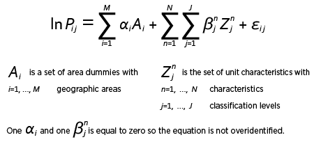
| Characteristics (n) | Classification levels (j) | |
|---|---|---|
| Geographic areas | States (50 plus the District of Columbia) State portions (51 metropolitan and 48 nonmetropolitan) Metropolitan statistical areas (383 plus the U.S. nonmetropolitan portion) |
|
| Structure type by number of bedrooms | Structure type | Number of bedrooms |
| Mobile and other | 0+ | |
| Apartment (<= 9 units ) | 0, 1, 2, 3+ | |
| Apartment (10+ units) | 0, 1, 2, 3+ | |
| Attached house | 1, 2, 3, 4+ | |
| Detached house | 1, 2, 3, 4+ | |
| Total number of rooms | 1, 2, 3, 4, 5, 7, 8, 9+ | |
| Year built | 1939 or before 1940–1979 1980–1999 2000 or after |
|
| Urban versus rural | Rural, urban | |
| Utilities included | No, yes | |
Characteristic parameters can be interpreted as the percent change in the rental price when a specific characteristic is present compared to a reference from which it is absent. The parameter results appear reasonable (table 3). For example, parameters on structure type and number of bedrooms are highest for houses and apartments with two or more bedrooms and are lowest for housing units with one or no bedrooms. They are higher for units in urban areas than for those in rural areas, for units with a larger rather than smaller room count, and for units built since 1980 rather than for units built before 1980. The parameter is also higher for units in which the rent payment does not include utilities, possibly reflecting tenant preferences for individually metered services.
| Model parameters | Estimate | Error | t | Pr > |t| |
|---|---|---|---|---|
| Intercept | 7.006 | 0.023 | 306.5 | <.0001 |
| Area | ||||
| Alabama | −0.306 | 0.023 | −13.3 | <.0001 |
| Alaska | 0.433 | 0.029 | 15.1 | <.0001 |
| Arizona | 0.082 | 0.023 | 3.6 | 0.0003 |
| Arkansas | −0.323 | 0.024 | −13.7 | <.0001 |
| California | 0.564 | 0.022 | 25.7 | <.0001 |
| Colorado | 0.342 | 0.023 | 15.0 | <.0001 |
| Connecticut | 0.278 | 0.023 | 11.9 | <.0001 |
| Delaware | 0.125 | 0.028 | 4.5 | <.0001 |
| District of Columbia | 0.590 | 0.026 | 23.0 | <.0001 |
| Florida | 0.220 | 0.022 | 9.9 | <.0001 |
| Georgia | −0.050 | 0.022 | −2.2 | 0.0265 |
| Hawaii | 0.602 | 0.025 | 23.8 | <.0001 |
| Idaho | −0.097 | 0.025 | −3.8 | 0.0001 |
| Illinois | 0.129 | 0.022 | 5.8 | <.0001 |
| Indiana | −0.148 | 0.023 | −6.5 | <.0001 |
| Iowa | −0.131 | 0.024 | −5.5 | <.0001 |
| Kansas | −0.143 | 0.024 | −6.1 | <.0001 |
| Kentucky | −0.244 | 0.023 | −10.6 | <.0001 |
| Louisiana | −0.130 | 0.023 | −5.6 | <.0001 |
| Maine | 0.076 | 0.026 | 2.9 | 0.0037 |
| Maryland | 0.352 | 0.023 | 15.5 | <.0001 |
| Massachusetts | 0.352 | 0.023 | 15.6 | <.0001 |
| Michigan | −0.056 | 0.022 | −2.5 | 0.0123 |
| Minnesota | 0.113 | 0.023 | 4.9 | <.0001 |
| Mississippi | −0.312 | 0.024 | −13.0 | <.0001 |
| Missouri | −0.160 | 0.023 | −7.0 | <.0001 |
| Montana | −0.030 | 0.027 | −1.1 | 0.2655 |
| Nebraska | −0.137 | 0.024 | −5.6 | <.0001 |
| Nevada | 0.122 | 0.023 | 5.2 | <.0001 |
| New Hampshire | 0.309 | 0.026 | 12.0 | <.0001 |
| New Jersey | 0.417 | 0.022 | 18.6 | <.0001 |
| New Mexico | −0.066 | 0.025 | −2.7 | 0.0071 |
| New York | 0.431 | 0.022 | 19.5 | <.0001 |
| North Carolina | −0.072 | 0.022 | −3.2 | 0.0012 |
| North Dakota | −0.090 | 0.027 | −3.3 | 0.0009 |
| Ohio | −0.173 | 0.022 | −7.8 | <.0001 |
| Oklahoma | −0.203 | 0.023 | −8.7 | <.0001 |
| Oregon | 0.217 | 0.023 | 9.4 | <.0001 |
| Pennsylvania | 0.009 | 0.022 | 0.4 | 0.6953 |
| Rhode Island | 0.102 | 0.026 | 4.0 | <.0001 |
| South Carolina | −0.104 | 0.023 | −4.5 | <.0001 |
| South Dakota | −0.199 | 0.027 | −7.3 | <.0001 |
| Tennessee | −0.116 | 0.023 | −5.1 | <.0001 |
| Texas | 0.098 | 0.022 | 4.4 | <.0001 |
| Utah | 0.092 | 0.024 | 3.8 | 0.0001 |
| Vermont | 0.307 | 0.029 | 10.4 | <.0001 |
| Virginia | 0.240 | 0.023 | 10.6 | <.0001 |
| Washington | 0.333 | 0.023 | 14.8 | <.0001 |
| West Virginia | −0.333 | 0.025 | −13.1 | <.0001 |
| Wisconsin | −0.017 | 0.023 | −0.7 | 0.4564 |
| Wyoming | 0.000 | ...... | ...... | ...... |
| Urban versus rural | ||||
| Rural | −0.285 | 0.003 | −88.4 | <.0001 |
| Urban | 0.000 | ...... | ...... | ...... |
| Structure type by number of bedrooms | ||||
| Mobile and other, 0+ | −0.525 | 0.006 | −84.6 | <.0001 |
| Apartment (<=9 units), 0 | −0.392 | 0.013 | −29.7 | <.0001 |
| Apartment (<=9 units), 1 | −0.394 | 0.006 | −65.7 | <.0001 |
| Apartment (<=9 units), 2 | −0.235 | 0.005 | −45.0 | <.0001 |
| Apartment (<=9 units), 3+ | −0.209 | 0.006 | −37.2 | <.0001 |
| Apartment (10+ units), 0 | −0.293 | 0.012 | −24.7 | <.0001 |
| Apartment (10+ units), 1 | −0.299 | 0.006 | −51.5 | <.0001 |
| Apartment (10+ units), 2 | −0.056 | 0.005 | −10.4 | <.0001 |
| Apartment (10+ units), 3+ | −0.135 | 0.007 | −19.6 | <.0001 |
| Attached house, 1 | −0.424 | 0.012 | −36.1 | <.0001 |
| Attached house, 2 | −0.123 | 0.007 | −18.3 | <.0001 |
| Attached house, 3 | −0.025 | 0.007 | −3.8 | 0.0001 |
| Attached house, 4+ | −0.043 | 0.013 | −3.4 | 0.0006 |
| Detached house, 1 | −0.435 | 0.009 | −50.6 | <.0001 |
| Detached house, 2 | −0.258 | 0.006 | −46.1 | <.0001 |
| Detached house, 3 | −0.093 | 0.005 | −19.8 | <.0001 |
| Detached house, 4+ | 0.000 | ...... | ...... | ...... |
| Total number of rooms | ||||
| 1 | −0.274 | 0.013 | −21.6 | <.0001 |
| 2 | −0.174 | 0.008 | −22.2 | <.0001 |
| 3 | −0.231 | 0.007 | −32.9 | <.0001 |
| 4 | −0.241 | 0.007 | −36.1 | <.0001 |
| 5 | −0.197 | 0.006 | −30.5 | <.0001 |
| 6 | −0.150 | 0.006 | −23.3 | <.0001 |
| 7 | −0.092 | 0.007 | −13.6 | <.0001 |
| 8 | −0.050 | 0.008 | −6.6 | <.0001 |
| 9 or more | 0.000 | ...... | ...... | ...... |
| Utilities included | ||||
| No | 0.186 | 0.003 | 62.8 | <.0001 |
| Yes | 0.000 | ...... | ...... | ...... |
| Year built | ||||
| 1939 or before | −0.266 | 0.003 | −81.9 | <.0001 |
| 1940–1979 | −0.279 | 0.002 | −112.8 | <.0001 |
| 1980–1999 | −0.160 | 0.003 | −61.6 | <.0001 |
| 2000 or after | 0 | ...... | ...... | ...... |
| Summary statistics | Estimate | |||
| Model sum of squares1 | 4,816,000 | |||
| Error sum of squares1 | 14,460,000 | |||
| Root mean squared error | 5.26 | |||
| R2 | 0.25 | |||
| Coefficient of variation | 78.49 | |||
| Observations used1 | 522,900 | |||
- Rounded to four significant digits.
Area parameters, (ai) in the model, measure rents price levels across regions. Along with separately estimated rents expenditure weights, these are aggregated with the price levels and weights of other consumption categories to estimate an overall RPP for each area.10 In addition to these all items RPPs, BEA also publishes three component RPPs that cover goods, rents, and other services. Component RPPs are estimated for the United States as well as for each area (table 4). All RPPs are indexed to the U.S. all items RPP, equal to 100.0.
Any pair of RPPs can be compared by evaluating their ratio.11 In 2017, the U.S. RPP for rents was 101.2, meaning across the United States, the price level for rents was 1.2 percent higher than the national average for all goods and services. Across states, Hawaii had the highest rents RPP (156.4), and West Virginia had the lowest RPP (61.4). Hawaii’s rents RPP is 54.5 percent higher than the national average price level for rents (101.2) and is 154.7 percent higher than West Virginia’s RPP.
Across states, rents RPPs generally increase with the share of population residing in the metropolitan portion (chart 1). The metropolitan portion comprises all counties within the state that belong to a metropolitan statistical area (MSA).12 These population shares range from 30.7 percent in Wyoming, where less than one-third of residents live in an MSA, to 100.0 percent in Delaware, New Jersey, and Rhode Island, where all residents reside in an MSA. In the District of Columbia, the share is also 100.0 percent. The national average is 85.9 percent.

[Click chart to expand]
Across states and large metropolitan areas—34 MSAs with a population greater than 2 million—rents RPPs were highest in the Mideast and Far West regions and were lowest in the Southeast, Great Lakes, and Mideast regions (tables 4 and 5).13
Hawaii had the highest rents RPP (156.4) across states. Its population is concentrated in the Urban Honolulu, HI MSA, on the island of Oahu, a location that constrains the amount of land available for housing. California had the second highest rents RPP (150.6) across states. The rents RPP in the District of Columbia was 154.5. In California and the District of Columbia, the population share living in an MSA is very high—97.9 percent and 100.0 percent, respectively.
Across large metropolitan areas—34 MSAs with a population greater than 2 million—the three highest rents RPPs were in California: San Francisco-Oakland-Hayward, CA (195.0), San Diego-Carlsbad, CA (168.0), and Los Angeles-Long Beach-Anaheim, CA (165.9).
State rents RPPs were lowest in the Southeast region. West Virginia had the lowest rents RPP (61.4), followed by Arkansas (62.1), and Mississippi (62.8). In these states, the population share living in an MSA is considerably smaller than the national average, ranging from 46.3 percent in Mississippi to 62.2 percent in Arkansas.
Large metropolitan areas with the lowest rents RPPs are in the Great Lakes, Southeast, and Mideast regions. Cleveland-Elyria, OH, had the lowest result (77.2), followed by Cincinnati, OH-KY-IN (78.7), and Pittsburgh, PA (79.4).
| Regional price parities | Population shares (percent) | |||||||
|---|---|---|---|---|---|---|---|---|
| All items | Goods | Services | Metropolitan portion | Nonmetropolitan portion | ||||
| Rents | Other | |||||||
| Total | Metropolitan portion | Nonmetropolitan portion | ||||||
| United States1 | 100.0 | 99.4 | 101.2 | 107.2 | 65.3 | 100.0 | 85.9 | 14.1 |
| Alabama | 86.7 | 96.5 | 63.1 | 66.5 | 47.8 | 93.3 | 76.5 | 23.5 |
| Alaska | 104.4 | 101.4 | 132.1 | 137.6 | 112.9 | 95.6 | 67.7 | 32.3 |
| Arizona | 96.4 | 96.8 | 93.0 | 95.8 | 51.8 | 98.4 | 95.0 | 5.0 |
| Arkansas | 86.5 | 94.9 | 62.1 | 68.1 | 48.6 | 93.3 | 62.2 | 37.8 |
| California | 114.8 | 103.5 | 150.6 | 153.6 | 98.1 | 107.0 | 97.9 | 2.1 |
| Colorado | 103.2 | 99.6 | 120.7 | 125.9 | 91.7 | 97.7 | 87.4 | 12.6 |
| Connecticut | 108.0 | 104.0 | 113.1 | 114.3 | 111.1 | 109.0 | 94.9 | 5.1 |
| Delaware2 | 100.1 | 98.9 | 97.1 | 97.8 | ...... | 103.3 | 100.0 | ...... |
| District of Columbia2 | 116.9 | 105.6 | 154.5 | 157.5 | ...... | 109.5 | 100.0 | ...... |
| Florida | 99.9 | 98.5 | 106.7 | 108.5 | 83.9 | 96.9 | 96.6 | 3.4 |
| Georgia | 92.5 | 96.9 | 81.6 | 87.5 | 54.3 | 95.2 | 82.9 | 17.1 |
| Hawaii | 118.5 | 111.3 | 156.4 | 168.4 | 110.2 | 103.2 | 80.9 | 19.1 |
| Idaho | 93.0 | 98.5 | 77.7 | 81.2 | 66.9 | 96.7 | 73.4 | 26.6 |
| Illinois | 98.5 | 98.3 | 97.5 | 103.3 | 58.1 | 99.2 | 88.5 | 11.5 |
| Indiana | 89.8 | 96.2 | 73.9 | 77.0 | 60.4 | 92.7 | 78.1 | 21.9 |
| Iowa | 89.8 | 95.0 | 75.2 | 82.6 | 62.2 | 90.9 | 59.6 | 40.4 |
| Kansas | 90.0 | 95.7 | 74.2 | 80.1 | 61.0 | 92.6 | 68.2 | 31.8 |
| Kentucky | 87.9 | 94.6 | 67.1 | 73.8 | 53.7 | 93.1 | 58.9 | 41.1 |
| Louisiana | 90.1 | 96.8 | 75.2 | 79.5 | 51.3 | 93.3 | 83.8 | 16.2 |
| Maine | 98.4 | 98.6 | 92.5 | 99.9 | 74.2 | 101.6 | 59.3 | 40.7 |
| Maryland | 109.4 | 103.6 | 121.8 | 124.8 | 81.6 | 106.8 | 97.5 | 2.5 |
| Massachusetts | 107.9 | 101.8 | 121.8 | 123.7 | 93.7 | 106.0 | 98.6 | 1.4 |
| Michigan | 93.0 | 97.4 | 81.0 | 83.3 | 68.2 | 95.3 | 82.0 | 18.0 |
| Minnesota | 97.5 | 101.3 | 96.0 | 103.6 | 70.1 | 94.1 | 77.8 | 22.2 |
| Mississippi | 85.7 | 94.1 | 62.8 | 72.4 | 51.5 | 93.3 | 46.3 | 53.7 |
| Missouri | 89.5 | 95.5 | 73.0 | 78.5 | 54.4 | 92.3 | 74.7 | 25.3 |
| Montana | 94.6 | 99.4 | 83.1 | 90.1 | 75.8 | 94.7 | 35.2 | 64.8 |
| Nebraska | 89.6 | 95.2 | 74.7 | 81.5 | 60.4 | 91.1 | 65.3 | 34.7 |
| Nevada | 97.6 | 95.9 | 96.8 | 98.8 | 85.3 | 100.5 | 90.8 | 9.2 |
| New Hampshire | 105.8 | 100.9 | 116.7 | 120.2 | 107.5 | 104.8 | 62.9 | 37.1 |
| New Jersey2 | 112.9 | 102.0 | 130.0 | 132.0 | ...... | 114.8 | 100.0 | ...... |
| New Mexico | 93.3 | 97.0 | 80.2 | 87.0 | 65.9 | 99.1 | 67.1 | 32.9 |
| New York | 115.8 | 108.8 | 131.8 | 136.5 | 78.9 | 113.1 | 93.1 | 6.9 |
| North Carolina | 91.3 | 96.6 | 79.7 | 83.2 | 61.8 | 93.3 | 78.5 | 21.5 |
| North Dakota | 90.1 | 94.8 | 78.3 | 80.6 | 73.8 | 90.8 | 50.4 | 49.6 |
| Ohio | 88.9 | 95.8 | 72.1 | 74.6 | 61.1 | 91.7 | 79.8 | 20.2 |
| Oklahoma | 89.0 | 95.8 | 69.9 | 74.9 | 56.9 | 93.3 | 67.5 | 32.5 |
| Oregon | 99.5 | 99.1 | 106.4 | 112.2 | 79.4 | 95.9 | 83.8 | 16.2 |
| Pennsylvania | 97.9 | 99.4 | 86.4 | 89.7 | 61.6 | 102.9 | 88.6 | 11.4 |
| Rhode Island2 | 98.6 | 98.4 | 94.9 | 95.7 | ...... | 101.5 | 100.0 | ...... |
| South Carolina | 90.4 | 96.9 | 77.2 | 80.3 | 54.0 | 93.3 | 85.2 | 14.8 |
| South Dakota | 88.2 | 94.7 | 70.2 | 79.9 | 59.7 | 90.7 | 48.4 | 51.6 |
| Tennessee | 90.4 | 96.4 | 76.3 | 80.7 | 56.9 | 93.3 | 77.6 | 22.4 |
| Texas | 97.0 | 97.1 | 94.5 | 98.2 | 65.1 | 98.5 | 89.2 | 10.8 |
| Utah | 97.0 | 96.6 | 93.9 | 96.3 | 82.2 | 99.6 | 89.5 | 10.5 |
| Vermont | 102.5 | 98.5 | 116.4 | 129.5 | 101.8 | 101.4 | 35.0 | 65.0 |
| Virginia | 102.1 | 99.8 | 108.9 | 116.5 | 59.5 | 100.5 | 87.7 | 12.3 |
| Washington | 106.4 | 104.4 | 119.5 | 124.2 | 85.7 | 101.6 | 90.0 | 10.0 |
| West Virginia | 87.0 | 94.6 | 61.4 | 62.0 | 55.7 | 94.9 | 61.8 | 38.2 |
| Wisconsin | 92.4 | 95.8 | 84.2 | 87.9 | 70.8 | 92.9 | 74.1 | 25.9 |
| Wyoming | 95.2 | 99.2 | 85.7 | 90.3 | 81.9 | 95.3 | 30.7 | 69.3 |
| Maximum | 118.5 | 111.3 | 156.4 | 168.4 | 112.9 | 114.8 | 100.0 | 69.3 |
| Minimum | 85.7 | 94.1 | 61.4 | 62.0 | 47.8 | 90.7 | 30.7 | 1.4 |
| Range | 32.8 | 17.2 | 95.0 | 106.4 | 65.1 | 24.1 | 69.3 | 67.8 |
- The U.S. all items regional price parity is the average price level across all states and the District of Columbia.
- All counties in Delaware, the District of Columbia, New Jersey, and Rhode Island are metropolitan.
| Regional price parities | ||||
|---|---|---|---|---|
| All items | Goods | Services | ||
| Rents | Other | |||
| United States1 | 100.0 | 99.0 | 101.8 | 100.1 |
| U.S. nonmetropolitan portion | 87.5 | 94.2 | 63.3 | 93.7 |
| Atlanta-Sandy Springs-Roswell, GA | 96.8 | 98.4 | 94.8 | 96.4 |
| Austin-Round Rock, TX | 100.5 | 98.1 | 119.4 | 93.5 |
| Baltimore-Columbia-Towson, MD | 107.2 | 103.1 | 114.7 | 105.7 |
| Boston-Cambridge-Newton, MA-NH | 111.8 | 102.3 | 140.8 | 107.1 |
| Charlotte-Concord-Gastonia, NC-SC | 93.8 | 97.6 | 87.5 | 93.5 |
| Chicago-Naperville-Elgin, IL-IN-WI | 103.4 | 99.3 | 113.9 | 102.3 |
| Cincinnati, OH-KY-IN | 90.0 | 95.1 | 78.7 | 91.3 |
| Cleveland-Elyria, OH | 90.2 | 95.8 | 77.2 | 91.8 |
| Columbus, OH | 92.3 | 96.0 | 84.5 | 92.2 |
| Dallas-Fort Worth-Arlington, TX | 100.2 | 98.7 | 105.9 | 98.8 |
| Denver-Aurora-Lakewood, CO | 106.3 | 100.5 | 133.4 | 98.0 |
| Detroit-Warren-Dearborn, MI | 95.8 | 98.7 | 86.2 | 98.5 |
| Houston-The Woodlands-Sugar Land, TX | 101.7 | 95.3 | 104.3 | 107.7 |
| Indianapolis-Carmel-Anderson, IN | 92.0 | 96.1 | 83.2 | 92.3 |
| Kansas City, MO-KS | 93.1 | 96.6 | 82.4 | 95.4 |
| Las Vegas-Henderson-Paradise, NV | 97.5 | 95.0 | 96.8 | 101.5 |
| Los Angeles-Long Beach-Anaheim, CA | 117.1 | 104.4 | 165.9 | 106.3 |
| Miami-Fort Lauderdale-West Palm Beach, FL | 108.4 | 101.6 | 130.0 | 101.5 |
| Minneapolis-St. Paul-Bloomington, MN-WI | 102.2 | 104.5 | 110.4 | 95.9 |
| New York-Newark-Jersey City, NY-NJ-PA | 122.3 | 109.4 | 153.1 | 117.7 |
| Orlando-Kissimmee-Sanford, FL | 98.3 | 98.1 | 105.8 | 93.5 |
| Philadelphia-Camden-Wilmington, PA-NJ-DE-MD | 105.4 | 100.7 | 109.6 | 108.2 |
| Phoenix-Mesa-Scottsdale, AZ | 97.7 | 96.2 | 98.9 | 98.5 |
| Pittsburgh, PA | 94.0 | 98.4 | 79.4 | 96.4 |
| Portland-Vancouver-Hillsboro, OR-WA | 101.7 | 99.0 | 120.6 | 95.8 |
| Riverside-San Bernardino-Ontario, CA | 107.2 | 100.2 | 117.8 | 107.4 |
| Sacramento—Roseville—Arden-Arcade, CA | 102.0 | 95.0 | 119.1 | 101.5 |
| St. Louis, MO-IL | 91.4 | 94.9 | 82.4 | 92.3 |
| San Antonio-New Braunfels, TX | 94.4 | 97.8 | 90.3 | 93.5 |
| San Diego-Carlsbad, CA | 116.0 | 98.6 | 168.0 | 107.1 |
| San Francisco-Oakland-Hayward, CA | 128.0 | 112.2 | 195.0 | 113.5 |
| Seattle-Tacoma-Bellevue, WA | 111.8 | 107.3 | 138.5 | 103.9 |
| Tampa-St. Petersburg-Clearwater, FL | 98.9 | 95.2 | 103.9 | 100.6 |
| Washington-Arlington-Alexandria, DC-VA-MD-WV | 118.4 | 105.3 | 164.4 | 109.8 |
| Maximum | 128.0 | 112.2 | 195.0 | 117.7 |
| Minimum | 90.0 | 94.9 | 77.2 | 91.3 |
| Range | 38.0 | 17.3 | 117.8 | 26.4 |
- The U.S. all items regional price parity is the average price level across all metropolitan areas and the U.S. nonmetropolitan portion.
- RPPs are calculated for the 50 states and the District of Columbia, metropolitan areas, and state metropolitan and nonmetropolitan portions. Estimates for metropolitan areas include an estimate for the nonmetropolitan portion of the United States to provide complete coverage of all U.S. counties.
- For a listing of CPI expenditure categories, see chapter 17 of the Handbook of Methods on the Bureau of Labor Statistics website.
- For a description of methods used to reconcile the CPI geographies with states and metropolitan areas, see Real Personal Income and Regional Price Parities on the BEA website.
- For ACS sample size data, see the Census website. For housing units, see American FactFinder.
- For a description of methods used to estimate rents expenditure weights, see Real Personal Income and Regional Price Parities on the BEA website.
- See note 5 above.
- For more information on ACS variable, see 2008 Subject Definitions on the Census website.
- The hedonic model with the utilities indicator yields rents price levels that control for differences between contract rent observations with utilities and for those without. For estimating all items RPPs, the price levels and expenditures for utilities are calculated separately using CPI data. The results are included in the housing category.
- This approach has been used in other federal government analyses of regional price levels. For example, see this 2002 Federal Register study to set regional salary levels.
- The aggregation combines 16 expenditure classes composed of 9 categories—apparel, education, food, housing, medical, recreation, rents, transportation, and other—subdivided into goods and services. Apparel consists only of goods, rents consists only of services, and the other seven categories consist of both goods and services.
- RPPs are independently estimated for states, metropolitan areas, and state metropolitan and nonmetropolitan portions. They can be compared within but not across geographies. It is incorrect to compare a state RPP with a state portion RPP.
- A metropolitan statistical area consists of a core county or group of counties in which there is an urban area with a population of at least 50,000 plus adjacent counties with a high degree of social and economic integration as measured through commuting ties.
- For a listing of states by BEA region, see the BEA website.