

The statistics discussed in this Regional Quarterly Report include the following: (1) local area gross domestic product (GDP) statistics for 2018, which were released officially by the Bureau of Economic Analysis (BEA) in December for the first time, (2) local area personal income (LAPI) statistics for 2018 and updated LAPI statistics for 1998–2017, and (3) personal consumption (PCE) expenditures by state for 2018.
Michael Bentley, Joshua Ingber, and Nayana Kollanthara prepared the sections on local area GDP and LAPI. Terence Fallon, Joshua Ingber, Solomon Kublashvili, and Steven Zemanek prepared the section on PCE by state.
On December 12, 2019, BEA released both current- and real-dollar statistics on local area (county) GDP for 2018. This is the first official release of county-level GDP, defined as the value of goods and services produced within a county. The size of a county's economy as measured by GDP varies considerably across the United States. In 2018, the total level of real GDP ranged from $18.4 million in Issaquena County, MS, to $710.9 billion in Los Angeles County, CA.
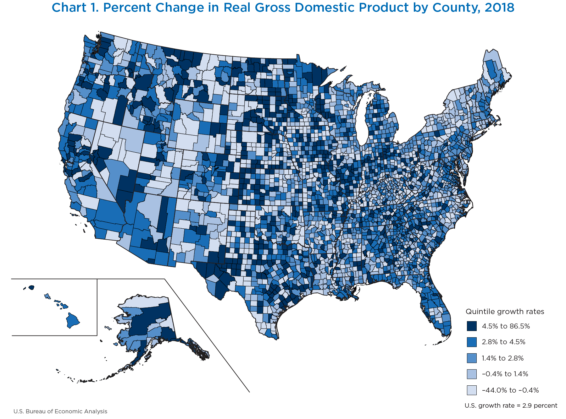
Chart 1 illustrates the percent change in GDP by county in 2018. GDP increased in 2,375 counties, decreased in 717 counties, and was unchanged in 21 counties in 2018. The percent change in GDP ranged from 86.5 percent in Jackson County, WV, to −44.0 percent in Grant County, ND. Details about the release are available on BEA’s website in the news release on county GDP estimates,1 and a detailed methodology is set for release in the February 2020 issue of the Survey of Current Business.
[Click chart to expand]
County-level GDP serves as an economic indicator measuring the economic vitality of local areas. However, since production is sometimes separated geographically from labor markets, it is helpful to consider another BEA indicator alongside GDP—local area personal income (LAPI). Personal income is defined as the income received by, or on behalf of, all persons from all sources—from participation as laborers in production, from owning a home or business, from the ownership of financial assets, and from government and business in the form of transfers. It includes income from domestic sources as well as from the rest of the world. For more on the methodology or definition, please see BEA’s LAPI methodology paper.2
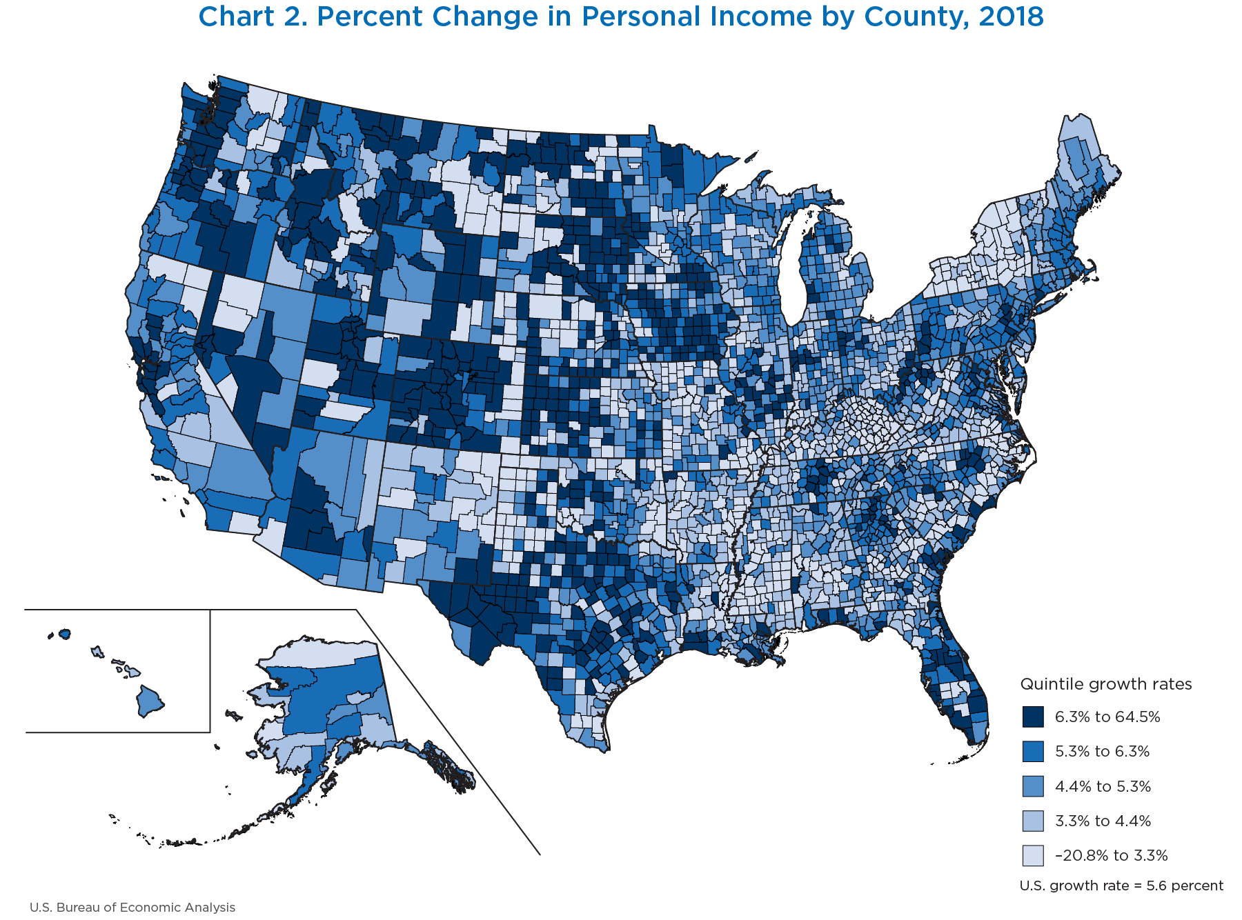
On November 14, 2019, BEA released current-dollar statistics on local area personal income. In 2018, total dollar levels of personal income ranged from $8.6 million in Loving County, TX, to $628.8 billion in Los Angeles County, CA. Chart 2 illustrates the percent change in personal income by county in 2018. Personal income increased in 3,019 counties, decreased in 91 counties, and was unchanged in 3 counties. The percent change in personal income ranged from −20.8 percent in Sherman County, TX, to 64.5 percent in Issaquena County, MS.
[Click chart to expand]
Considered together, personal income and GDP offer powerful insights into the local economy. It is possible to use both personal income and GDP as measures of recovery from the Great Recession (2008–2009), when national GDP declined, and a majority of counties experienced a decline in GDP as well.
Tables 1 and 2 describe the top 10, the median, and the bottom 10 counties by average growth rates, using a geometric mean of growth, for GDP and personal income, respectively. Karnes County, TX, leads all counties in GDP growth, increasing its productivity, on average, 46.8 percent in the decade following the recession.
| Total GDP by county(thousands of dollars)1 | Total GDP by county, average growth rate for 2009–2018 (percent) | ||
|---|---|---|---|
| 2009 | 2018 | ||
| Karnes, TX | 418,454 | 13,268,891 | 46.8 |
| La Salle, TX | 360,216 | 7,785,896 | 40.7 |
| Reeves, TX | 657,168 | 12,656,413 | 38.9 |
| Dimmit, TX | 358,735 | 5,904,287 | 36.5 |
| Doddridge, WV | 127,267 | 1,354,094 | 30.0 |
| McMullen, TX | 369,088 | 3,730,348 | 29.3 |
| Culberson, TX | 161,776 | 1,599,940 | 29.0 |
| Loving, TX | 1,001,378 | 9,556,632 | 28.5 |
| Glasscock, TX | 584,186 | 5,443,954 | 28.1 |
| Gonzales, TX | 613,153 | 4,960,284 | 26.1 |
| Median2 (Motley, TX) | 37,208.61 | 41,465.80 | 1.2 |
| Freestone, TX | 3,356,543 | 1,382,934 | −9.4 |
| Ohio, IN | 260,487 | 103,661 | −9.7 |
| Knott, KY | 552,407 | 210,606 | −10.2 |
| Johnson, WY | 1,152,513 | 438,751 | −10.2 |
| Clay, WV | 285,753 | 108,545 | −10.2 |
| Boone, WV | 1,774,533 | 663,183 | −10.4 |
| Roberts, TX | 2,897,356 | 1,015,484 | −11.0 |
| Terrell, TX | 512,394 | 161,791 | −12.0 |
| Zapata, TX | 2,604,696 | 819,217 | −12.1 |
| St. John the Baptist, LA | 14,567,820 | 2,361,164 | −18.3 |
- Source. U.S. Bureau of Economic Analysis
- The median county is defined as that ranked 1,557th of the 3,113 counties.
| Total personal income by county (thousands of dollars)1 | Total personal income by county, average growth rate for 2009–2018 (percent) | ||
|---|---|---|---|
| 2009 | 2018 | ||
| Loving, TX | 2,234 | 8,623 | 16.2 |
| Glasscock, TX | 39,676 | 141,777 | 15.2 |
| McKenzie, ND | 248,500 | 852,673 | 14.7 |
| Billings, ND | 23,678 | 68,633 | 12.6 |
| Midland, TX | 8,513,490 | 21,478,156 | 10.8 |
| Wasatch, UT | 732,667 | 1,771,209 | 10.3 |
| Benton, AR | 10,293,948 | 24,232,084 | 10.0 |
| Hudspeth, TX | 66,559 | 155,701 | 9.9 |
| Sumter, FL | 2,554,076 | 5,935,589 | 9.8 |
| Karnes, TX | 342,820 | 776,133 | 9.5 |
| Median2 (Bingham, ID) | 1,245,972 | 1,679,963 | 3.4 |
| Stephens, TX | 409,107 | 370,612 | −1.1 |
| Mora, NM | 178,840 | 160,116 | −1.2 |
| Atchison, MO | 247,429 | 220,457 | −1.3 |
| Carroll, KY | 442,783 | 390,274 | −1.4 |
| Hall, TX | 104,027 | 91,385 | −1.4 |
| Throckmorton, TX | 62,235 | 54,450 | −1.5 |
| Hancock, KY | 383,395 | 323,423 | −1.9 |
| Slope, ND | 45,714 | 37,750 | −2.1 |
| Ohio, IN | 289,555 | 237,932 | −2.2 |
| Issaquena, MS | 31,551 | 24,251 | −2.9 |
- Source. U.S. Bureau of Economic Analysis
- The median county is defined as that ranked 1,557th of the 3,113 counties
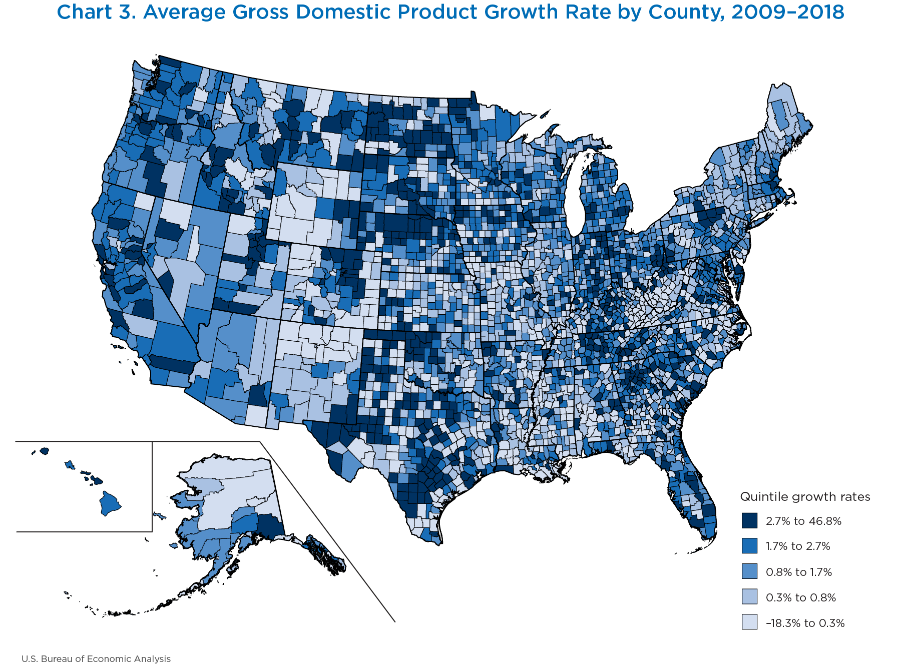
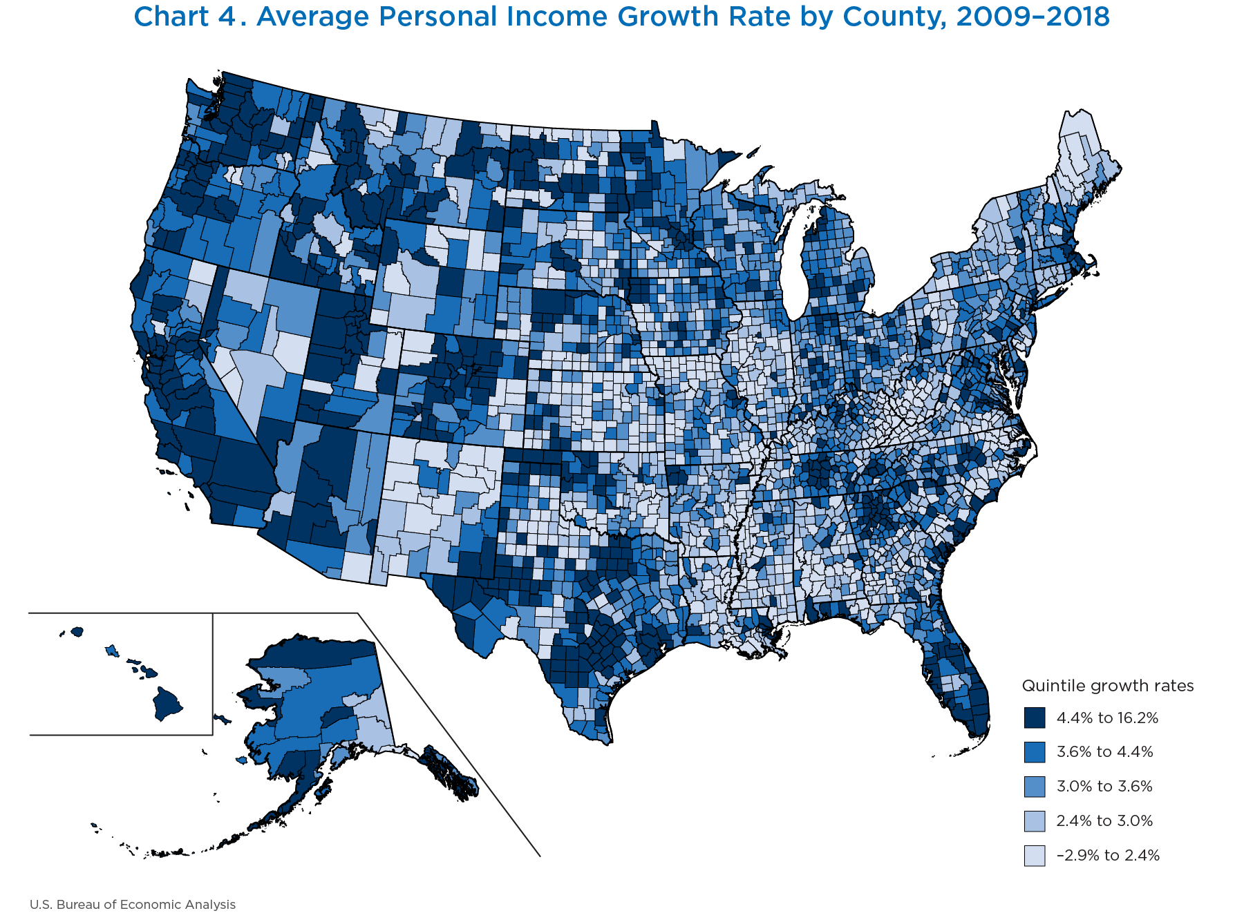
However, Karnes County was ranked 10th in income growth over the period, demonstrating some key differences between the two indicators: (1) geographic location of production and income are correlated but not necessarily aligned, and (2) growth in personal income, in accord with expectations and economic theory, lags that of GDP. Charts 3 and 4 map these growth rates to consider the possibility of a regional trend in growth over the period.
Many of the fastest and slowest growing counties, for both GDP and personal income, are found in Texas. Given the diverse economic makeup in Texas, it can serve as a microcosm for describing the types of counties and industries that contributed to the recovery. Also, restricting the analysis to Texas is helpful because counties in Texas share, for the most part, state-level institutional, legal, and cultural norms. Whereas, a comparison between a Texas county and, for example, a Minnesota county do not account for differences in taxation policy, property rights, or a multitude of other explanatory factors that help to understand growth.
[Click chart to expand]
[Click chart to expand]
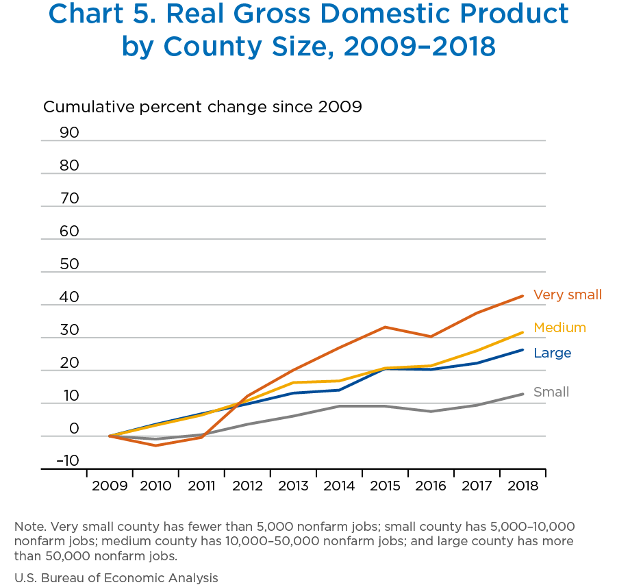
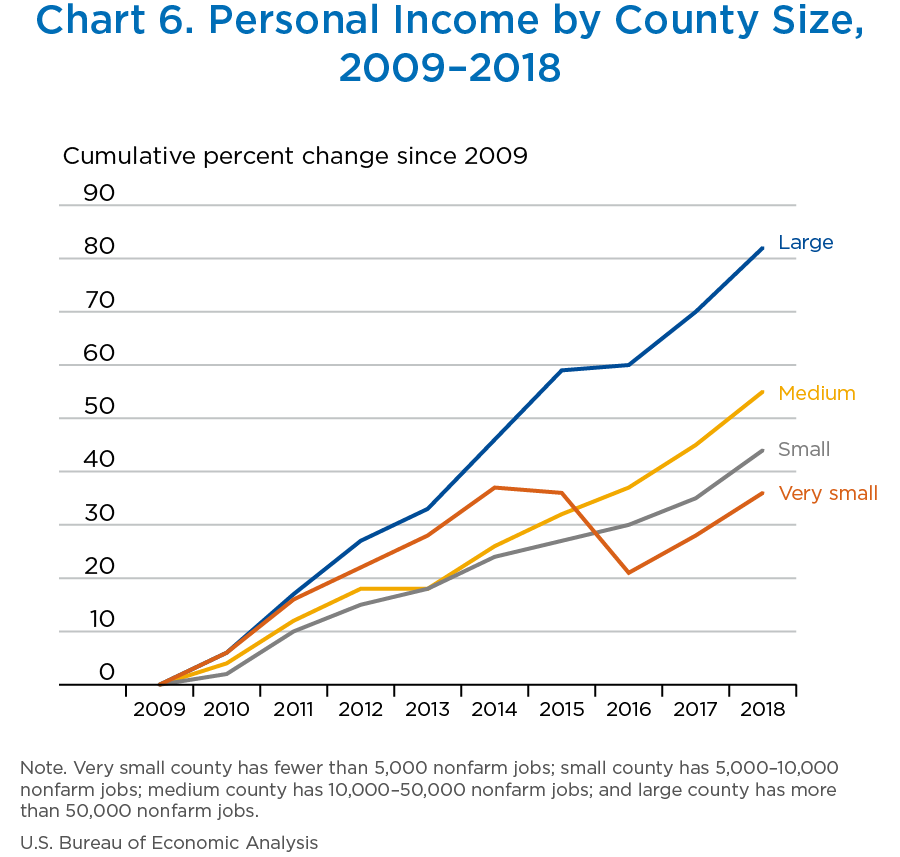
Counties bear some resemblance according to their size. Dividing Texas into counties with fewer than 5,000 nonfarm jobs (“very small”), 5,000 to 10,000 nonfarm jobs (“small”) 10,000 to 50,000 nonfarm jobs (“medium”), and more than 50,000 nonfarm jobs (“large”) allows for the consideration of county size as a factor for growth. Charts 5 and 6 depict percent changes in real GDP and current-dollar personal income for all counties in Texas, with 2009 as a base year.
[Click chart to expand]
Interestingly, we see that very small Texas counties had the highest percent change in GDP over the period, 42.7 percent, despite a delayed start to the growth. Very small counties had higher rates of GDP growth than small counties (12.8 percent), medium counties (31.6 percent), and large counties (26.3 percent) over the period. On one hand, very small counties would expect larger percent changes, as a small increase in GDP magnifies the effect on calculating a percent change, when GDP is already small. However, we do not see this effect in small counties, nor is it present when looking at personal income. In addition, economic theory suggests that productivity gains occur when people specialize and trade, a feature of denser locations. Thus, despite expectation, the smallest Texas counties increased their productivity at rates higher than larger counties. Most likely, this growth can be traced to the decade’s boom in mining, quarrying, and oil and gas extraction. Property rights in Texas are such that land owners can lease their land to bigger production firms, who benefit from economies of scale in the production process. Thus, small producers, who traditionally can only participate in a market when they are priced-in by high market prices for oil, gas, or mining extract, can circumvent the impact of price fluctuations by leasing out their land.
[Click chart to expand]
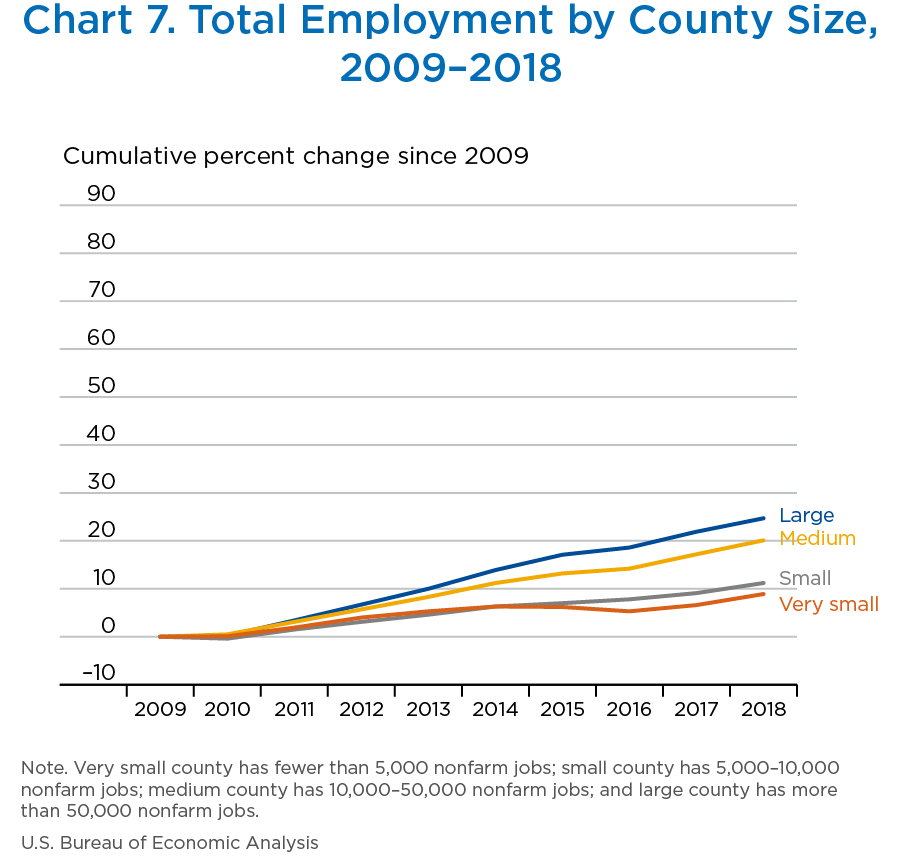
When looking at personal income, the data better conform to economic expectations. The largest counties experience an 82.3 percent increase in personal income. We see that very small counties grew significantly during the first half of the decade, almost keeping pace with their larger state counterparts. Eventually, we see an income distribution effect according to size; where medium counties grew 55.3 percent, small counties 44.0 percent, and very small counties 35.5 percent. Similarly, job growth is distributed by size as well, as seen in chart 7. Keeping the same scale across these charts reveals some indication that income is outpacing job growth.
[Click chart to expand]
Different industries or different sources of income contribute to overall growth and provide another framework to understand the recovery period. To highlight this, consider how certain industries drove growth in GDP and different sources of income drove growth in personal income in Karnes and Zapata counties, TX. Karnes County benefitted from the fastest average GDP growth in the state, 46.8 percent. In addition, its average personal income growth was 9.6 percent. Conversely, Zapata County experienced the most dramatic average decline in GDP in the state, −12.1 percent. Despite declines in GDP, average growth in personal income in Zapata County was 2.8 percent.
Karnes County, Texas
Karnes County, a very small county, is located in the southeastern part of Texas, approximately 50 miles southeast of San Antonio, TX, and had a population of 15,650 in 2018. It sits on the Eagle Ford Shale, which ranks as one of the largest oil and gas developments in the world, based on capital investment. It has been reported that approximately $30 billion was spent developing oil and gas extraction in the Eagle Ford Shale area.
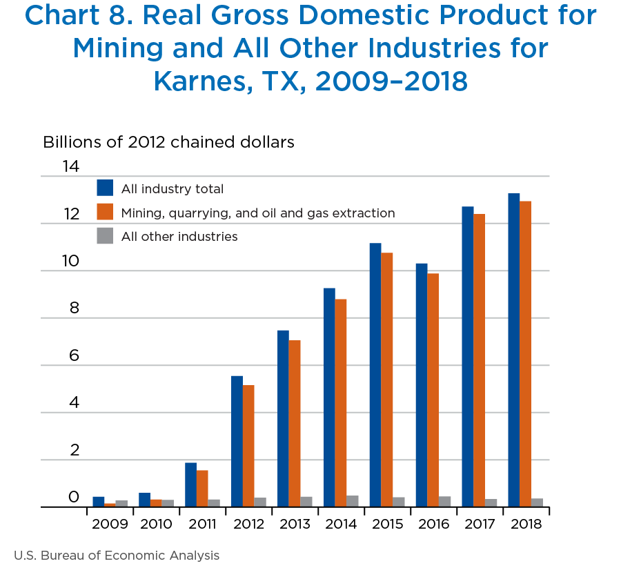
Average GDP growth in Karnes County from 2009 to 2018 was 46.8 percent. Chart 8 shows the GDP growth of all industries in Karnes County as well as the growth of the mining, quarrying, and oil and gas extraction industry. The all other industries category includes industries such as agriculture, forestry, fishing, and hunting; construction; manufacturing; wholesale and retail trade; and arts, entertainment, and recreation. As shown in chart 8, the largest contribution to overall real GDP growth in Karnes County from 2009 to 2018 can be primarily attributed to the mining, quarrying, and oil and gas extraction industry due to the Eagle Ford Shale boom in the county.
[Click chart to expand]
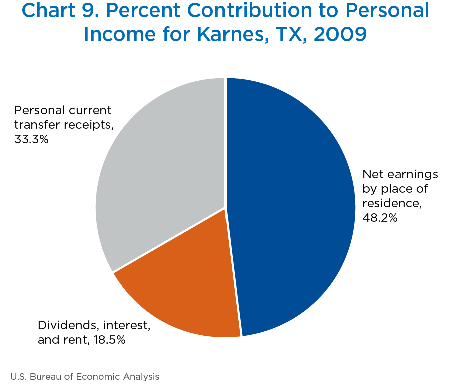
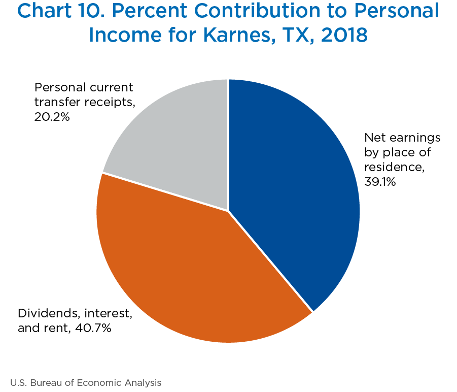
Average personal income growth in Karnes County from 2009 to 2018 was 9.6 percent. Charts 9 and 10 show the percent contribution of the three major components of personal income in Karnes County for both 2009 and 2018. In Karnes County, dividends, interest, and rent, which includes royalties, contributed 18.5 percent in 2009 but accounted for 40.7 percent of personal income in 2018; while personal current transfer receipts and net earnings by place of residence decreased over the 10-year period. The driver of personal income growth was dividends, interest, and rent, which supports the notion that Karnes County residents leased land to firms in the mining, quarrying, and oil and gas extraction sector.
[Click chart to expand]
[Click chart to expand]
Zapata County, Texas
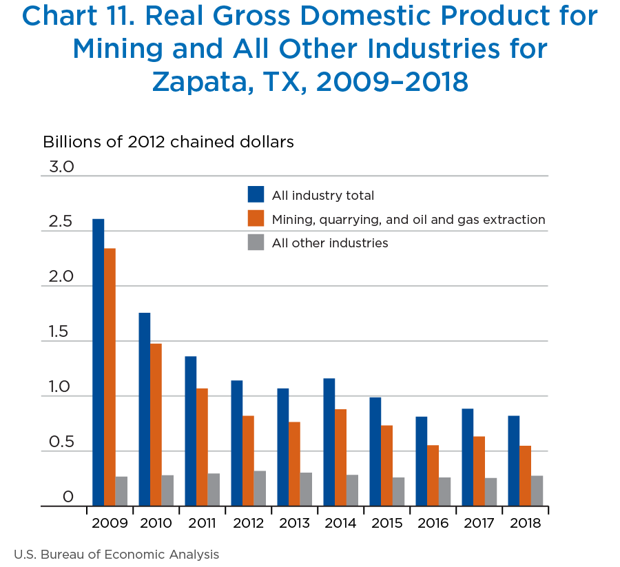
Average GDP declined in Zapata County from 2009 to 2018 and was −12.1 percent. Chart 11 shows the magnitude of which the mining, quarrying, and oil and gas extraction industry contributed to the overall GDP decline in Zapata County. It also shows real GDP for all other industries combined.
Zapata county, also a very small county, located in southern Texas along the U.S.-Mexico border, had a population of 14,190 in 2018. Oil was discovered in Zapata County in 1919, during the Texas oil boom of the early 20th century. Over the past 10 years Zapata County has experienced a decline in oil production as oil deposits have been depleted in the county, alternative areas of oil extraction have been developed in other parts of Texas and the country, and the price of oil has decreased to the point of making oil wells in Zapata County unprofitable. However, the mining, quarrying, and oil and gas extraction industry is still important in Zapata County, as natural gas production is significant there, accounting for approximately 0.7 percent of overall natural gas production in Texas.
[Click chart to expand]
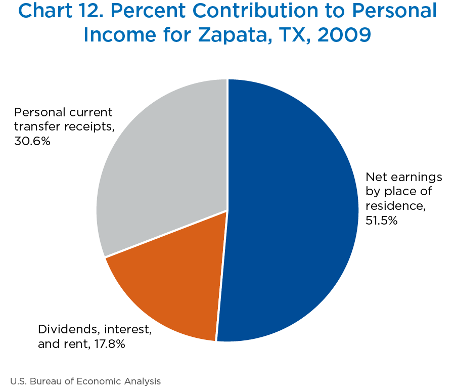
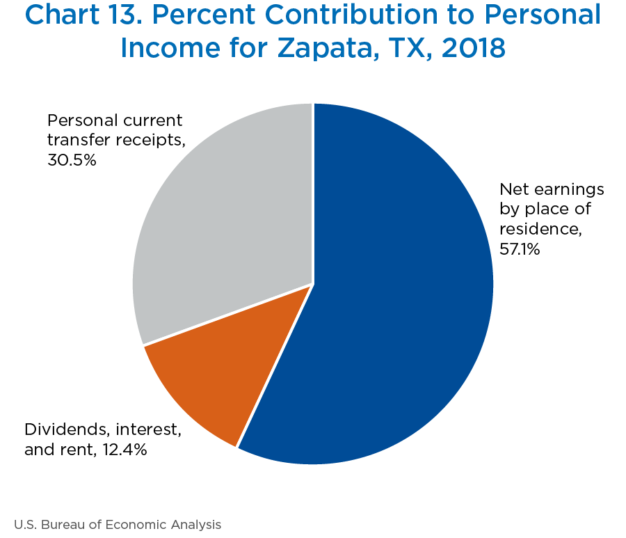
In contrast, average growth in personal income in Zapata County from 2009 to 2018 was 2.8 percent. Charts 12 and 13 show the percent contribution of the three major components of personal income in Zapata County for both 2009 and 2018. Net earnings by place of residence, income earned from labor, contributed to the growth of personal income from 2009 to 2018 in Zapata. In 2009, this component contributed 51.5 percent to personal income; it contributed 57.1 percent in 2018. Personal current transfer receipts didn’t show any significant change, while dividends, interest, and rent decreased from 17.8 percent in 2009 to 12.4 percent in 2018.
[Click chart to expand]
[Click chart to expand]
Earnings in the mining, quarrying, and oil and gas extraction industry was the leading contributor to overall earnings growth in Zapata County, as natural gas production increased over the last 10 years. However, dividends, interest, and rents decreased most likely as royalties, a part of rents, declined because oil production has significantly decreased in the county. Oil production in Zapata County has decreased due to economic substitution, as oil production in Texas has shifted to the Eagle Ford Shale and the Permian Basin.
Methodology, source data, and revisions
GDP by county
On December 12, 2019, BEA released the first official measures of GDP by county. GDP can be measured as the sum of income payments and other costs incurred in the production of goods and services. This “income approach” to measuring GDP is conceptually equivalent to the production approach that measures gross output minus intermediate inputs and the final expenditures approach that measures the sum of personal consumption, private investment, government spending, and exports less imports. As with BEA GDP by state statistics, the county statistics employ the income approach to measuring GDP; that is, GDP is computed as the sum of compensation of employees, taxes on production and imports less subsidies, and gross operating surplus, as shown here:
GDPcnty,i = Compensationcnty,i + Taxes on Production and Imports less Subsidiescnty,i + Gross Operating Surpluscnty,i
BEA produces county-level statistics for the compensation of employees and the proprietors’ income portion of gross operating surplus in its estimation of county-level personal income. By a simple rearrangement of terms, a residual component of GDP, representing the sum of (1) gross operating surplus minus proprietors’ income and (2) taxes on production and imports less subsidies, can be calculated. It is this residual component of GDP that needs to be estimated to complete the measurement of GDP by county, as shown here:
GDPcnty,i = Compensationcnty,i + Proprietors’ incomecnty,i + (Gross Operating Surplus less Proprietors’ income + Taxes on Production and Imports less Subsidies)cnty,i
GDP by county is published at the sector level, however, many industries are estimated at the three-digit North American Industry Classification System (NAICS) level. To estimate the county residual portion of GDP for each industry, BEA first calculates the state-level residual value for each industry from BEA GDP by state statistics. County-level industry source data are used as indicators to distribute the calculated state-level residual portion for each industry to produce county estimates. The resulting county statistics sum to published GDP by state by industry.
The source data fall into one of two categories—general or industry-specific. General data sources capture data on all published industries and were incorporated into the methodology for most industries, while industry-specific data sources were incorporated into one industry. Tables 3 and 4 list the two categories of data sources the industries that rely upon those data.
| Industry | Economic Census | National Establishment Time Series | Additional sources of data used |
|---|---|---|---|
| Agriculture, forestry, fishing, and hunting1 | ✓ | ||
| Mining1 | ✓ | ||
| Utilities | |||
| Construction2 | ✓ | ||
| Manufacturing | ✓ | ✓ | |
| Wholesale trade | ✓ | ✓ | |
| Retail trade | ✓ | ✓ | |
| Transportation and warehousing1 | ✓ | ✓ | ✓ |
| Information | ✓ | ✓ | |
| Finance and insurance1 | ✓ | ✓ | ✓ |
| Real estate and rental and leasing1 | ✓ | ✓ | ✓ |
| Professional and technical services | ✓ | ✓ | |
| Management of companies and enterprises | |||
| Administrative and waste services | ✓ | ✓ | |
| Educational services | ✓ | ✓ | |
| Health care and social assistance | ✓ | ✓ | |
| Arts, entertainment, and recreation | ✓ | ✓ | |
| Accommodation and food services | ✓ | ✓ | |
| Other services, except government | ✓ | ✓ | |
| Government1 | ✓ |
- Denotes additional source data in the sub-industry detail.
- Denotes additional source data at the sector level.
| Industry | Additional source data |
|---|---|
| Agriculture, forestry, fishing, and hunting | |
| Farms | Bureau of Economic Analysis (BEA) farm receipts and expenses |
| Mining data | |
| Oil and gas extraction | Drilling Edge |
| Mining except oil and gas extraction | Energy Information Agency (EIA) |
| Construction | Dodge Analytics |
| Transportation and warehousing | |
| Air transportation | Bureau of Transportation Statistics |
| Rail transportation | Amtrak Surface Transportation Board |
| Finance and insurance | |
| Banking | Federal Deposit Insurance Corporation |
| Real estate and rental and leasing | |
| Real estate | BEA imputed rent, BEA rental income from farms owned by nonoperator landlords, American Housing Survey |
| Government | |
| Federal civilian | Bureau of Labor Statistics (BLS), EIA |
| Federal military | BLS |
Chained-dollar values of GDP by county are derived by applying national chain-type price indexes to the current-dollar values of GDP by county for 65 detailed NAICS-based industries. The chain-type index formula that is used in the national accounts is then used to calculate the values of total real GDP by county and real GDP by county at more aggregated industry levels.
Because of the sensitivity of some of the source data used in estimation, the GDP by county statistics are subject to suppressions via disclosure avoidance of confidential source data. These suppressions have been applied according to the guidance accompanying any sensitive source data. A full discussion of the methodology is forthcoming in the February 2020 Survey of Current Business.
Local area personal income
Each November, BEA typically revises the annual local areal personal income estimates to incorporate the results of the July annual update of the National Income and Product Accounts,3 to incorporate the results of the September annual update of state personal income,4 and to incorporate revised source data that are more complete and more detailed than those previously available. With the November 14, 2019, release of local area personal income, the annual estimates for 1998–2017 were revised. The revisions for 1998–2013 were solely due to revisions to state estimates of personal interest income as a result from an improvement in the estimation methodology and data sources.
The main 2018 county-level data used by BEA to prepare the estimates of local area personal income presented in this article were wage and salary data from the Bureau of Labor Statistics, benefits paid by the Social Security Administration, Medicare enrollment and fee-for-service expenditure data from the Centers for Medicare and Medicaid Services, and Medicaid payments from state departments of social services. In addition, Internal Revenue Service tabulations of 2017 federal income tax returns were used, primarily for dividends, interest, nonfarm proprietors’ income, and the residence adjustment.5 Other county-level data were used to prepare estimates of various components of local area personal income, including the following (table 5):
- For local area farm income, farm cash receipts, government payments, crop production, livestock stocks, and crop insurance indemnity payments by county for 2018 from the U.S. Department of Agriculture and state offices of agricultural statistics were used.
- For military earnings, the number of full-time military and Coast Guard personnel by county for 2018 from the Departments of Defense and Homeland Security was used.
- For state unemployment insurance compensation, county-level data for 2018 from state employment security agencies were used.
- For a few small components of personal income, population (excluding population in group quarters) by county for 2018 from the Census Bureau was used to allocate state estimates to the counties.
| Data | Source |
|---|---|
| Wages and salaries by industry | |
| In general | BLS Quarterly Census of Employment and Wages data |
| Farm | USDA Census of Agriculture data |
| Agriculture and forestry support activities | USDA Census of Agriculture data |
| Rail transportation | RRB payroll and employment data; Census Bureau Journey to Work (Census of Population) data |
| Educational services | Census Bureau County Business Patterns payroll data; state departments of education employment data; DOE Private School Universe Survey employment data; Official Catholic Directory number of teachers in religious orders data |
| Membership associations and organizations | Household population data2 |
| Private households | Household population data;2 Census Bureau Journey to Work (Census of Population) data |
| Military | DOD personnel data; DHS Coast Guard personnel and payroll data; household population data2 |
| State and local government | Census Bureau American Community Survey wage data; RRB payroll and employment data |
| Employer contributions for employee pension and insurance funds by industry | |
| All industries | BEA estimates of wages and employment3 |
| Employer contributions for government social insurance by industry | |
| All industries | BLS state unemployment insurance programs employer contributions data |
| Proprietors’ income | |
| Farm | USDA Census of Agriculture data; USDA National Agriculture and Statistic Service crop production and livestock stocks data; cash receipts from state offices of agricultural statistics; USDA Farm Service Agency and Natural Resource Conservation Service government payments to farmers data; USDA Risk Management Agency crop indemnity payments data |
| Nonfarm industries | IRS data on net profits of sole proprietorships and partnerships |
| Residence adjustment | Census Bureau Journey to Work (American Community Survey) employment and wage data; IRS wage data |
| Dividends, interest, and rent | IRS income tax returns data on dividends, taxable interest, and gross rents and royalties; OPM federal civilian retirement payments data; DOD military retirement payments data; Census Bureau Census of Housing data on the aggregate gross rental value of owner-occupied single-family dwellings and number of mobile homes; USDA gross rental value of farm dwellings data |
| Personal current transfer receipts | SSA Social Security and Supplemental Security Income enrollees and benefits data; CMS data on the number of enrollees in the Medicare Hospital Insurance, Supplementary Medical Insurance, and Part D programs; CMS Medicare Advantage fee-for-services expenditure data; data from the Treasury Department’s USASpending.gov (higher education student assistance and railroad worker retirement benefits); Census Bureau Small Area Income and Poverty Estimates (persons and children age 0–17 in poverty and number of Supplemental Nutritional Assistance Program recipients); Census Bureau American Indian and Alaska Native Alone population and household population data;2 DOD Tricare payments data; IRS refundable income tax credit data; number of unemployed persons from the BLS Local Area Unemployment Statistics program; DVA veterans pension, disability, life insurance, and readjustment benefits data and number of pension and disability beneficiaries; NSF federal fellowship benefits data; Federal Reserve Bank of New York data on the number of mortgage debtors, per debtor mortgage debt balance and percent of mortgage debt in delinquency; Medicaid payments, Children’s Health Insurance Program enrollment, Supplemental Nutritional Assistance Program benefits, energy assistance payments, general assistance benefits, and family assistance benefits data from the state departments of social services; state unemployment insurance compensation data from the state employment security agencies |
| Employee and self-employed contributions for government social insurance | CMS Medicare Parts B and D enrollment data; Census Bureau American Community Survey veteran population data; BEA estimates of employment |
- BEA prepares some county estimates by aggregating source data available by ZIP code.
- Household population for counties is calculated as the difference between the Census Bureau population and the Census Bureau population in group quarters estimates.
- See theLocal Area Personal Income Methodology for the data sources used by BEA to estimate employment.
- BEA
- Bureau of Economic Analysis
- BLS
- Bureau of Labor Statistics
- CMS
- Centers for Medicare and Medicaid Services
- DHS
- Department of Homeland Security
- DOD
- Department of Defense
- DOE
- Department of Education
- DVA
- Department of Veterans Affairs
- IRS
- Internal Revenue Service
- NSF
- National Science Foundation
- OPM
- Office of Personnel Management
- RRB
- Railroad Retirement Board
- SSA
- Social Security Administration
- USDA
- U.S Department of Agriculture
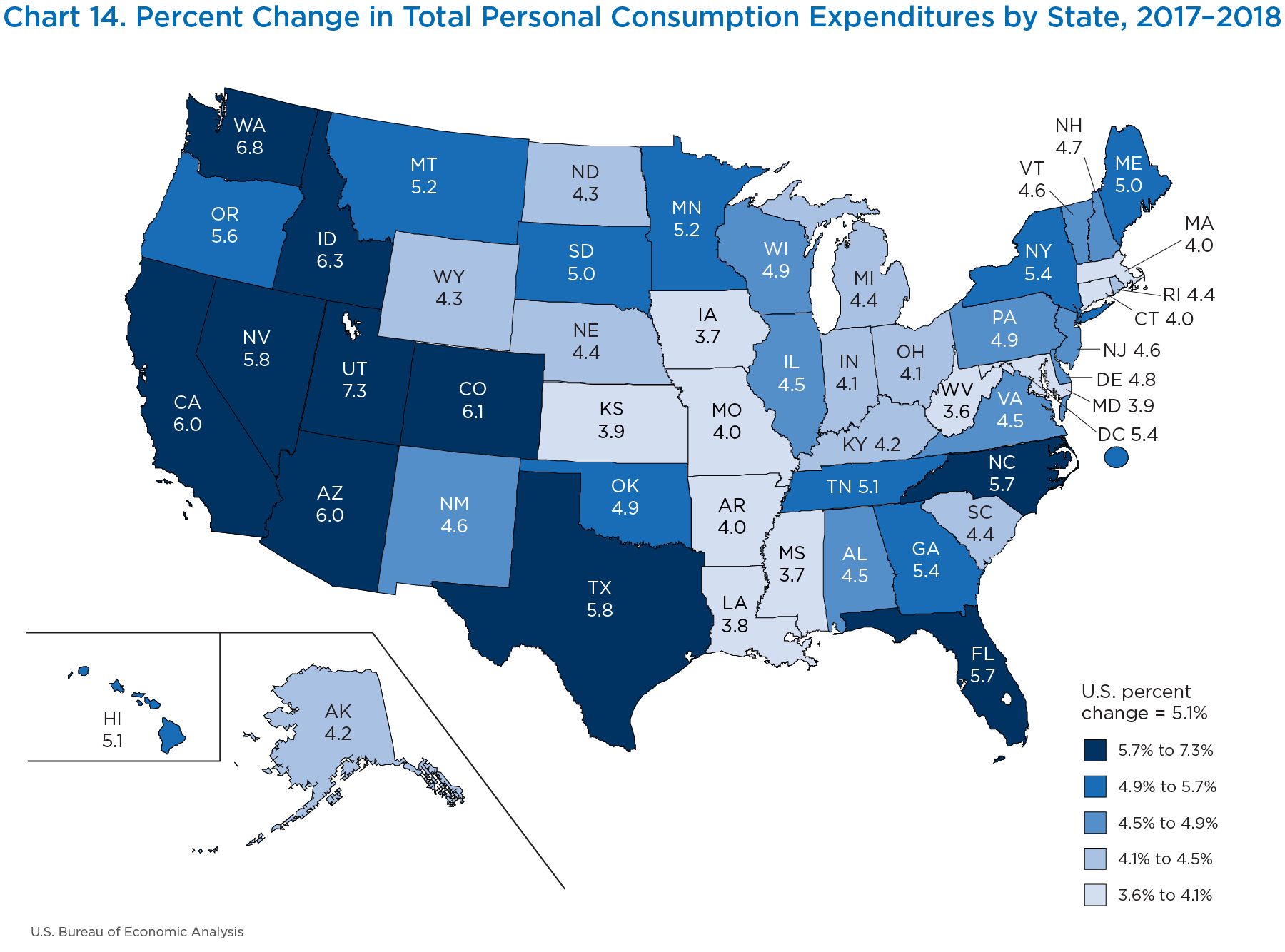
On October 3, 2019, BEA released current-dollar statistics on PCE by state for 2018. PCE grew 5.1 percent nationwide in 2018, increasing in all states and the District of Columbia. The percent change for the states ranged from a high of 7.3 percent in Utah to a low of 3.6 percent in West Virginia (chart 14).
[Click chart to expand]
PCE by state is a household consumption measure that reflects the value of the goods and services purchased by, or on behalf of, households by state of residence. These statistics on households provide an indication of economic well-being as well as information on consumption patterns across states and over time. For example, the statistics show how households allocate their spending between goods and services or between necessities and discretionary items or how consumers adjust their spending to changes in the economy.
Additionally, the 2018 statistics represent a 10-year period, from the Great Recession of 2009, when national current-dollar GDP and PCE were at low points compared to the prior year. In 2009, national current-dollar GDP decreased 1.8 percent and national current-dollar PCE decreased 1.3 percent from the preceding year.
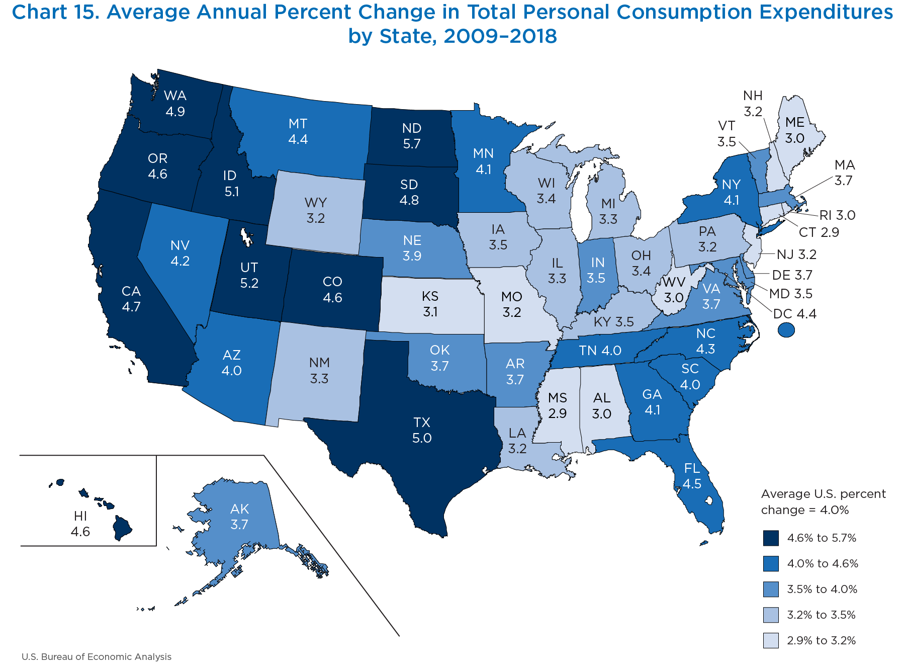
From 2009 to 2018, national PCE grew 4.0 percent on average, and like the 2018 PCE by state statistics, all states and the District of Columbia experienced PCE growth during this time. The states with the largest average percent change in PCE from 2009 to 2018 were in the western half of the United States. The fastest growing states were North Dakota, Utah, and Idaho, which increased 5.7 percent, 5.2 percent, and 5.1 percent, respectively. In contrast, the states with slowest average growth rates in PCE from 2009 to 2018 were concentrated in the New England and the Southeast regions. The slowest growing states on average were Mississippi, Connecticut, and Maine, which increased 2.9 percent, 2.9 percent, and 3.0 percent, respectively (chart 15).
[Click chart to expand]
North Dakota
North Dakota was the fastest growing state over the 2009–2018 time period, with PCE increasing on average 5.7 percent. Similar to the other high performing states, North Dakota’s average growth was driven by categories with large budget shares of total state PCE, such as housing and utilities, health care, and financial services and insurance.
North Dakota had several consumption categories that ranked among the fastest growing in the country. Housing and utilities expenditures grew at an average of 6.7 percent from 2009–2018, the fastest growth of any state during this time period. Health care expenditures grew at an average of 5.6 percent, the third fastest rate in the United States. Financial services and insurance was another standout category for North Dakota, with a 7.2 percent growth rate, the fourth fastest in the United States during this time period (table 6).
| Category | 2009 | 2018 | Average annual percent change |
|---|---|---|---|
| Personal consumption expenditures | 22,448 | 36,863 | 5.7 |
| Goods | 8,761 | 13,458 | 4.9 |
| Durable goods | 3,067 | 5,026 | 5.6 |
| Motor vehicles and parts | 1,079 | 1,876 | 6.3 |
| Furnishings and durable household equipment | 645 | 1,038 | 5.4 |
| Recreational goods and vehicles | 889 | 1,424 | 5.4 |
| Other durable goods | 454 | 689 | 4.7 |
| Nondurable goods | 5,694 | 8,431 | 4.5 |
| Food and beverages purchased for off-premises consumption | 1,696 | 2,423 | 4.0 |
| Clothing and footwear | 692 | 1,024 | 4.5 |
| Gasoline and other energy goods | 1,393 | 2,120 | 4.8 |
| Other nondurable goods | 1,914 | 2,863 | 4.6 |
| Services | 13,687 | 23,405 | 6.1 |
| Household consumption expenditures (for services) | 12,908 | 22,057 | 6.1 |
| Housing and utilities | 2,820 | 5,069 | 6.7 |
| Health care | 4,043 | 6,612 | 5.6 |
| Transportation services | 580 | 1,119 | 7.6 |
| Recreation services | 822 | 1,363 | 5.8 |
| Food services and accommodations | 1,381 | 2,284 | 5.8 |
| Financial services and insurance | 1,724 | 3,234 | 7.2 |
| Other services | 1,539 | 2,376 | 4.9 |
| Final consumption expenditures of nonprofit institutions serving households | 778 | 1,348 | 6.3 |
| Gross output of nonprofit institutions | 2,124 | 3,527 | 5.8 |
| Less: Receipts from sales of goods and services by nonprofit institutions | 1,345 | 2,179 | 5.5 |
Note. Percent change from preceding period was calculated from unrounded data. Expenditures may not sum to higher level aggregates because of rounding.
Housing and utilities expenditures include rents paid by tenants for tenant-occupied housing, imputed rental values for owner-occupied housing, rental value of farm dwellings, spending on group housing, and spending on utilities consisting of water supply, sanitation, electricity, and gas. Health care expenditures include spending on outpatient services, hospital, and nursing home services. Outpatient services consist of physician services, dental services, and paramedical services. Health care services do not include pharmaceuticals or medical products, as these are classified in other nondurable goods. Financial services and insurance expenditures consist of spending on financial service charges, fees, and commissions as well as an imputed value for financial services furnished without payment. Insurance expenditures consist of life insurance, net household insurance, net health insurance, net motor vehicle insurance, and other transportation insurance.
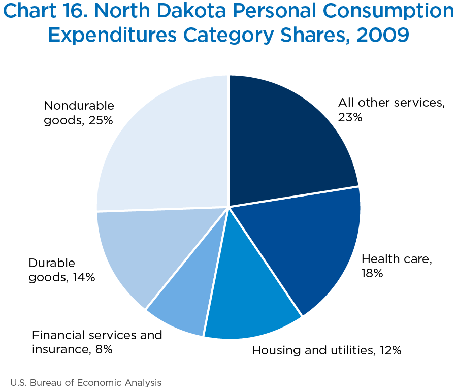
These categories were among the largest contributors to growth in North Dakota, and they comprised the largest portion of total PCE for the state. In 2009, housing and utilities, health care, and financial services and insurance combined to make 38 percent of total PCE. In 2018, these three categories increased their share to 41 percent at the expense of the goods categories, which include purchases like groceries and gasoline (charts 16 and 17).
[Click chart to expand]

[Click chart to expand]
The strong growth in North Dakota was also evident in BEA state personal income and GDP statistics. During the 2009–2018 period, nominal personal income had an average annual growth rate of 6.0 percent, and nominal GDP had an average annual growth rate of 7.5 percent, while nationally, personal income and GDP grew at a rate of 4.4 percent and 4.0 percent, respectively (chart 18).
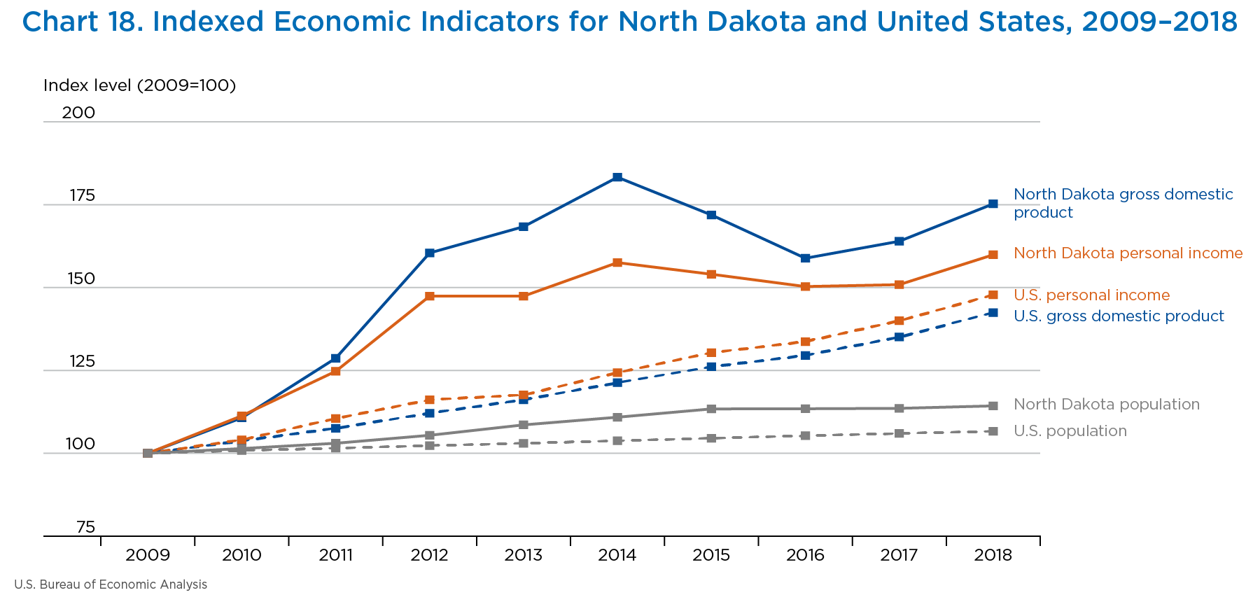
[Click chart to expand]
When evaluating personal income and GDP statistics, it is important to consider their measure and scope. Personal income by state is the income received by, or on behalf of, all persons from all sources—from participation as laborers in production, from owning a home or business, from the ownership of financial assets, and from government and business in the form of transfers. Personal income by state is measured on a place-of-residence basis. GDP by state is the value of goods and services produced by the labor and property located in a state. GDP by state is measured on a place-of-work basis.
The oil boom in North Dakota played a central role in the state’s economic performance over the period. The boom began in the mid-2000s with the discovery of the Parshall field in the Bakken formation. The discovery and subsequent mining expansion helped mitigate the effects of the Great Recession in 2009, as oil and gas extraction continued to accelerate into the early 2010s. The oil boom contributed to the state’s economic expansion in several ways, including a population increase, as people flocked to the state to fill jobs. During this time, North Dakota had among the lowest rates of unemployment in the country. In turn, the increase in population fueled other aspects of the economy, including housing construction, personal income, and PCE.
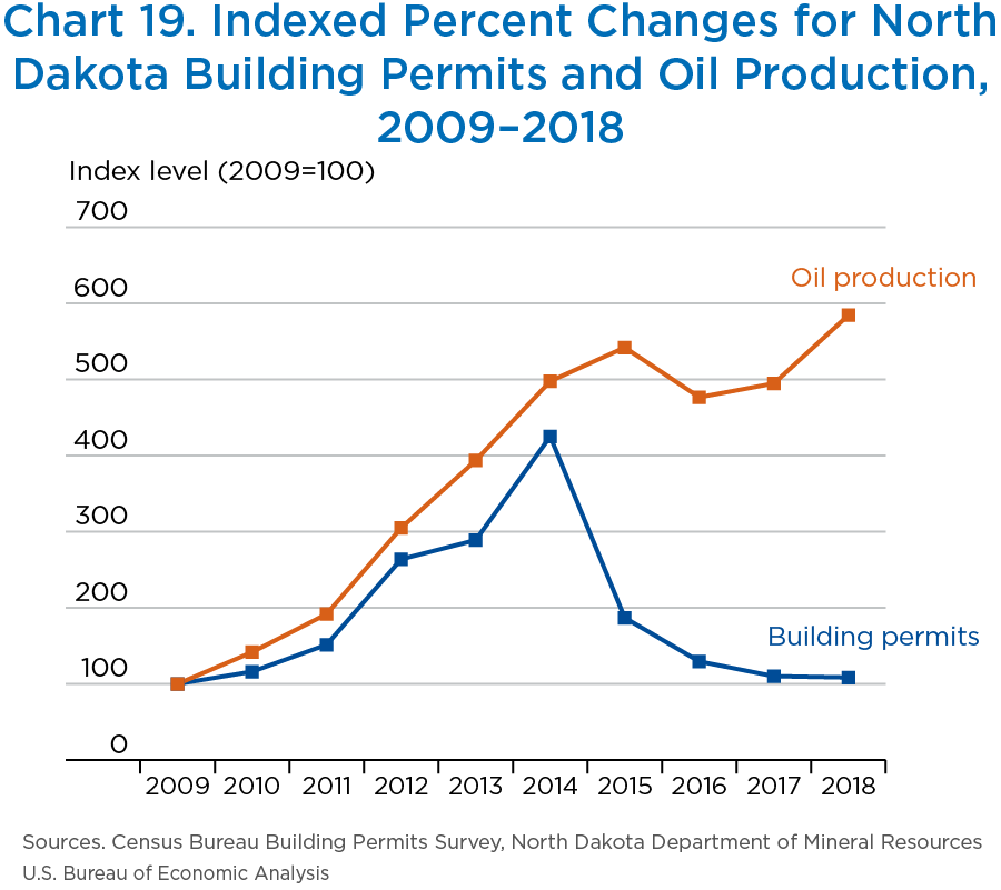
The average growth in PCE matched the expansion of oil production in North Dakota during that time period. Oil production increased every year from 2009 to 2015, with a slight dip in 2016, followed by expansion again in 2018. Overall, oil production increased at a strong average annual growth rate of 48.4 percent (chart 19). During the same period, more workers found housing in the state. Building permits for new housing increased each year until a spike in 2014, resulting in an average annual growth rate of 32.5 percent from 2009–2014. Building permits then decreased as fewer houses were built from 2014–2018. The average annual growth rate of building permits from 2009–2018 was 0.8 percent.
[Click chart to expand]
Connecticut
Connecticut was among the slowest growing states for the 2009–2018 time period, with PCE increasing 2.9 percent on average. Connecticut’s slow growth was emblematic of other states in the same region, including Rhode Island and Maine. A common characteristic for the slow growth was an underperforming category with a large budget share of total state PCE, such as housing and utilities or health care.
Expenditures on housing and utilities in Connecticut had a modest average growth rate of 2.6 percent from 2009 to 2018. In contrast, the average national growth rate for housing and utilities expenditures was 3.5 percent, while North Dakota, the fastest growing state, boasts a growth rate of 6.7 percent during the same period. Similarly, the growth rate for expenditures on health care in Connecticut was 2.5 percent, while nationally, expenditures on health care services had a growth rate of 4.1 percent. Other categories contributing to the slow growth were expenditures on food and beverages purchased for off-premises consumption, which grew 2.2 percent, and expenditures on clothing and footwear, which grew 1.3 percent. Furthermore, Connecticut was the only state with a PCE category that decreased in value over the 2009–2018 period. The average growth rate of expenditures on gasoline and other energy goods decreased an average of 0.4 percent (table 7).
| Category | 2009 | 2018 | Average annual percent change |
|---|---|---|---|
| Personal consumption expenditures | 145,915 | 189,141 | 2.9 |
| Goods | 43,401 | 54,377 | 2.5 |
| Durable goods | 13,535 | 17,609 | 3.0 |
| Motor vehicles and parts | 4,105 | 5,713 | 3.7 |
| Furnishings and durable household equipment | 3,343 | 4,320 | 2.9 |
| Recreational goods and vehicles | 3,912 | 4,985 | 2.7 |
| Other durable goods | 2,175 | 2,591 | 2.0 |
| Nondurable goods | 29,866 | 36,769 | 2.3 |
| Food and beverages purchased for off-premises consumption | 9,981 | 12,147 | 2.2 |
| Clothing and footwear | 4,169 | 4,674 | 1.3 |
| Gasoline and other energy goods | 3,703 | 3,574 | −0.4 |
| Other nondurable goods | 12,013 | 16,374 | 3.5 |
| Services | 102,514 | 134,764 | 3.1 |
| Household consumption expenditures (for services) | 97,442 | 127,567 | 3.0 |
| Housing and utilities | 30,415 | 38,235 | 2.6 |
| Health care | 22,580 | 28,186 | 2.5 |
| Transportation services | 4,902 | 6,671 | 3.5 |
| Recreation services | 5,782 | 7,212 | 2.5 |
| Food services and accommodations | 7,186 | 10,182 | 3.9 |
| Financial services and insurance | 12,431 | 18,159 | 4.3 |
| Other services | 14,147 | 18,921 | 3.3 |
| Final consumption expenditures of nonprofit institutions serving households | 5,072 | 7,196 | 4.0 |
| Gross output of nonprofit institutions | 19,011 | 25,425 | 3.3 |
| Less: Receipts from sales of goods and services by nonprofit institutions | 13,939 | 18,229 | 3.0 |
Note. Percent change from preceding period was calculated from unrounded data. Expenditures may not sum to higher level aggregates because of rounding.
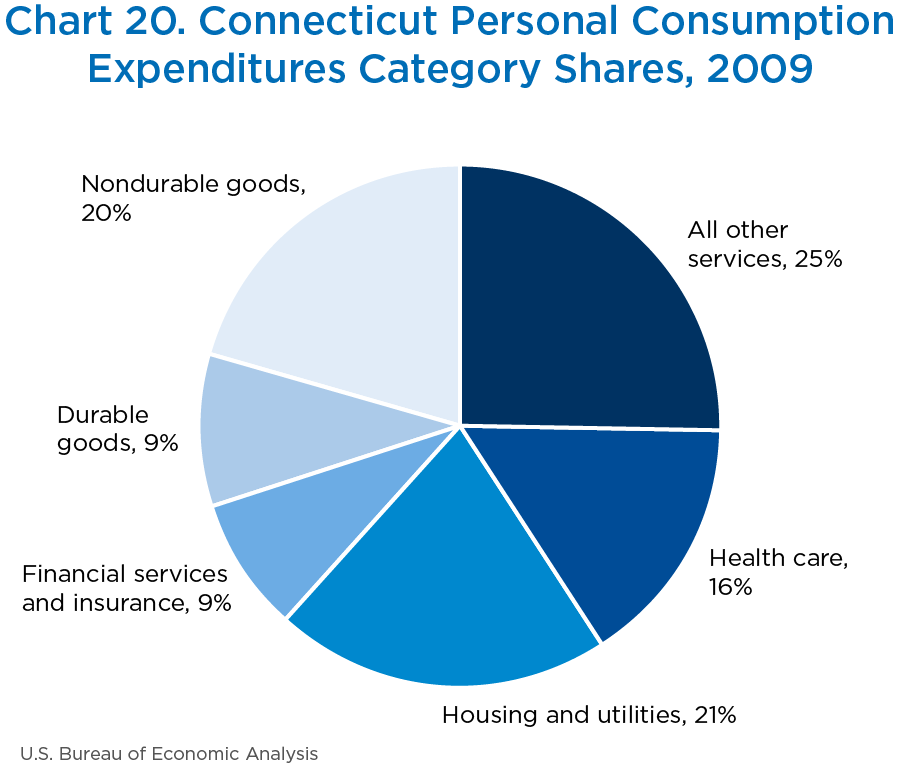
In 2009, housing and utilities and health care were 37 percent of the total expenditures—the largest detail categories based on current-dollar expenditures. However, the share of expenditures had decreased to 35 percent of the total in 2018. Meanwhile, nondurable goods, which includes gasoline and other energy goods, had a 20 percent share of total PCE in 2009, but the share decreased to 19 percent of total state PCE in 2018 (charts 20 and 21).
[Click chart to expand]

[Click chart to expand]
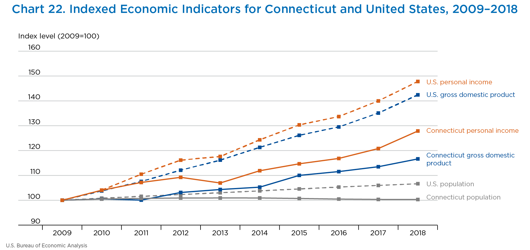
The slow growth in Connecticut was also evident in BEA personal income, GDP, and population statistics. During the 2009–2018 period, personal income had a growth rate of 2.8 percent, and GDP grew 1.7 percent, while nationally, personal income and GDP grew at a rate of 4.4 percent and 4.0 percent, respectively. Connecticut has a larger than average share of its economy associated with the finance and insurance industries compared to the U.S. average. These industries were affected disproportionally during the Great Recession. While these industries have recovered nationally since then, the pace of the recovery has not been as fast as in Connecticut. During the 2009–2018 period, GDP growth in the finance and insurance industry in Connecticut increased 0.9 percent compared to 5.5 percent for the nation, while earnings (the portion of personal income earned by laborers) in finance and insurance in Connecticut increased 0.5 percent compared to 4.1 percent for the nation. The slow recovery in finance and insurance has kept the overall average growth in Connecticut below average for many of the state’s economic indicators (chart 22).
[Click chart to expand]
Connecticut’s population growth was another factor affecting its economy. The state’s population growth was below the national average over the last 10 years, including the last 5 years, when the population declined. There are three components of a state’s population change: natural change (difference between births and deaths), net domestic migration (difference between U.S. residents moving to and leaving a state), and net international migration (difference between non-U.S. residents moving to and leaving a state). The primary contributor to Connecticut’s population change was net domestic migration. While natural change in Connecticut was consistent with the overall national trend, the net domestic migration trend for the 2009–2018 period showed more residents were leaving the state than could be replaced by the other components (table 8).
| Year | Population change | Natural change | Net domestic migration | Net international migration |
|---|---|---|---|---|
| 2009 | 15,356 | 12,170 | −7,824 | 11,322 |
| 2010 | 4,978 | 2,649 | 124 | 2,452 |
| 2011 | 8,898 | 8,327 | −12,343 | 13,027 |
| 2012 | 6,372 | 7,766 | −17,392 | 16,035 |
| 2013 | 520 | 6,354 | −16,929 | 11,171 |
| 2014 | −132 | 6,490 | −25,041 | 18,263 |
| 2015 | −7,274 | 5,946 | −29,986 | 16,614 |
| 2016 | −8,835 | 5,807 | −29,202 | 14,489 |
| 2017 | −4,794 | 4,327 | −23,652 | 14,454 |
| 2018 | −1,215 | 3,736 | −21,509 | 16,494 |
Source. U.S. Census Bureau
Revisions
The October release of PCE by state included updated statistics for 2014–2017. The updated statistics incorporated the results of the 2019 annual update of the National Income and Product Accounts and newly available and revised regional source data. Source data that were either revised or newly released included new and revised data from the Bureau of Labor Statistics Quarterly Census of Employment and Wages for 2014–2018 and new 2017 data from the Census Bureau American Community Survey (table 9).
| Component | Major sources | Updates and revisions |
|---|---|---|
| Durable goods; nondurable goods; some services | Economic Census; Quarterly Census of Employment and Wages (QCEW) | Revised QCEW 2014–2017, new 2018 |
| Housing and utilities | American Community Survey (ACS) | New 2017 ACS data |
| Owner-to-renter ratios from Regional Price Parity program | New owner-to-renters ratios based on the 2016 ACS panel (2012–2016) | |
| Economic Research Service data on imputed rental value of farm dwellings (for farm housing) | Revised 2016 and new 2017 price and volume data for electricity | |
| Water supply data from U.S. Geological Survey and National Association of Clean Water Agencies (NACWA) regional water price index | Revised 2016–2017 price and volume data for natural gas | |
| Volume and price data on electricity and natural gas consumption from the Energy Information Administration | Revised NACWA service charge index 2013–2017 | |
| Transportation services | Economic Census, QCEW | Revised QCEW 2014–2017, new 2018 |
| Amtrak ridership by state (rail transportation) | New data from the National Association of Rail Passengers 2017 | |
| Bureau of Transportation Statistics (BTS) passenger enplanement by state (air transportation) | Updated 2015–2017 BTS data | |
| Financial services and insurance | Federal Deposit Insurance Corporation (FDIC), National Credit Union Administration (NCUA), Internal Revenue Service (IRS), National Association of Insurance Commissioners (NAIC) | New 2017 data from FDIC, NCUA, IRS, NAIC |
| Health care services | Economic Census for some subcomponents, QCEW, Center for Medicare and Medicaid Services | Revised QCEW 2014–2017, new 2018 |
Current-dollar PCE nationwide was revised downward 0.1 percent for 2017 (table 10). The revisions ranged from a downward 0.5 percent in the District of Columbia to an upward 0.3 percent in South Dakota. Current-dollar PCE was revised downward in 30 states and the District of Columbia and was revised upward in 20 states. The revisions were due to new and revised source data, as there were no methodological improvements to the statistics.
| Revised PCE (millions of dollars) | Revision (millions of dollars) | Percent revision | ||||||||||
|---|---|---|---|---|---|---|---|---|---|---|---|---|
| 2014 | 2015 | 2016 | 2017 | 2014 | 2015 | 2016 | 2017 | 2014 | 2015 | 2016 | 2017 | |
| United States1 | 11,814,798 | 12,277,398 | 12,741,883 | 13,305,559 | −1,279 | −10,249 | −18,399 | −9,304 | 0.0 | −0.1 | −0.1 | −0.1 |
| New England | 675,701 | 698,931 | 720,066 | 748,738 | −225 | −618 | −1,012 | 307 | 0.0 | −0.1 | −0.1 | 0.0 |
| Connecticut | 167,846 | 172,191 | 176,126 | 181,887 | −123 | −255 | −246 | −105 | −0.1 | −0.1 | −0.1 | −0.1 |
| Maine | 52,972 | 54,214 | 55,700 | 57,989 | −28 | −75 | −139 | 59 | −0.1 | −0.1 | −0.2 | 0.1 |
| Massachusetts | 324,369 | 337,925 | 350,117 | 365,714 | −56 | −298 | −438 | 309 | 0.0 | −0.1 | −0.1 | 0.1 |
| New Hampshire | 61,286 | 63,074 | 64,884 | 67,534 | −2 | −13 | −82 | 39 | 0.0 | 0.0 | −0.1 | 0.1 |
| Rhode Island | 41,687 | 43,185 | 44,283 | 45,710 | −14 | 21 | −64 | −60 | 0.0 | 0.0 | −0.1 | −0.1 |
| Vermont | 27,541 | 28,342 | 28,955 | 29,904 | −2 | 2 | −42 | 65 | 0.0 | 0.0 | −0.1 | 0.2 |
| Mideast | 2,098,141 | 2,168,700 | 2,241,141 | 2,328,039 | −586 | −783 | −2,207 | −3,725 | 0.0 | 0.0 | −0.1 | −0.2 |
| Delaware | 36,814 | 38,195 | 39,313 | 40,711 | −26 | −45 | −40 | −28 | −0.1 | −0.1 | −0.1 | −0.1 |
| District of Columbia | 36,768 | 38,872 | 40,367 | 42,069 | −58 | −45 | −73 | −204 | −0.2 | −0.1 | −0.2 | −0.5 |
| Maryland | 243,828 | 252,947 | 261,760 | 272,369 | −89 | −12 | −306 | −187 | 0.0 | 0.0 | −0.1 | −0.1 |
| New Jersey | 409,845 | 423,080 | 435,270 | 449,237 | −134 | 291 | −346 | −240 | 0.0 | 0.1 | −0.1 | −0.1 |
| New York | 870,260 | 901,125 | 936,268 | 976,732 | −135 | −587 | −604 | −1,667 | 0.0 | −0.1 | −0.1 | −0.2 |
| Pennsylvania | 500,626 | 514,480 | 528,162 | 546,921 | −143 | −387 | −837 | −1,400 | 0.0 | −0.1 | −0.2 | −0.3 |
| Great Lakes | 1,694,766 | 1,749,160 | 1,804,437 | 1,876,027 | −111 | −1,359 | −3,153 | −1,490 | 0.0 | −0.1 | −0.2 | −0.1 |
| Illinois | 494,570 | 512,441 | 528,632 | 549,540 | −92 | −413 | −803 | −17 | 0.0 | −0.1 | −0.2 | 0.0 |
| Indiana | 217,291 | 223,339 | 231,053 | 242,122 | 67 | −36 | −278 | 81 | 0.0 | 0.0 | −0.1 | 0.0 |
| Michigan | 352,709 | 363,600 | 376,136 | 390,263 | −41 | −328 | −1,169 | −632 | 0.0 | −0.1 | −0.3 | −0.2 |
| Ohio | 418,262 | 431,446 | 442,596 | 458,883 | −112 | −287 | −705 | −498 | 0.0 | −0.1 | −0.2 | −0.1 |
| Wisconsin | 211,934 | 218,335 | 226,021 | 235,220 | 67 | −295 | −198 | −424 | 0.0 | −0.1 | −0.1 | −0.2 |
| Plains | 776,267 | 801,108 | 827,366 | 863,154 | −216 | −772 | −1,746 | −150 | 0.0 | −0.1 | −0.2 | 0.0 |
| Iowa | 107,281 | 110,378 | 113,876 | 118,533 | −16 | −76 | −346 | 90 | 0.0 | −0.1 | −0.3 | 0.1 |
| Kansas | 97,374 | 100,199 | 102,838 | 106,176 | −52 | −16 | −244 | −253 | −0.1 | 0.0 | −0.2 | −0.2 |
| Minnesota | 221,445 | 229,645 | 239,698 | 253,012 | −82 | −416 | −491 | 89 | 0.0 | −0.2 | −0.2 | 0.0 |
| Missouri | 214,401 | 220,915 | 226,997 | 235,905 | −138 | −317 | −516 | −194 | −0.1 | −0.1 | −0.2 | −0.1 |
| Nebraska | 68,812 | 71,138 | 74,009 | 77,068 | −7 | −29 | −118 | −43 | 0.0 | 0.0 | −0.2 | −0.1 |
| North Dakota | 34,315 | 34,943 | 34,603 | 35,353 | 90 | 87 | 16 | 66 | 0.3 | 0.2 | 0.0 | 0.2 |
| South Dakota | 32,640 | 33,891 | 35,345 | 37,107 | −11 | −5 | −45 | 95 | 0.0 | 0.0 | −0.1 | 0.3 |
| Southeast | 2,701,997 | 2,808,783 | 2,913,198 | 3,037,883 | −252 | −2,893 | −4,885 | −2,413 | 0.0 | −0.1 | −0.2 | −0.1 |
| Alabama | 145,877 | 149,687 | 153,224 | 158,574 | 81 | −59 | −233 | 199 | 0.1 | 0.0 | −0.2 | 0.1 |
| Arkansas | 88,427 | 91,127 | 94,581 | 98,838 | 4 | −74 | −132 | 72 | 0.0 | −0.1 | −0.1 | 0.1 |
| Florida | 723,031 | 762,444 | 793,162 | 829,401 | 102 | −665 | −904 | 0 | 0.0 | −0.1 | −0.1 | 0.0 |
| Georgia | 323,329 | 334,526 | 348,182 | 364,092 | −74 | −823 | −944 | −1,229 | 0.0 | −0.2 | −0.3 | −0.3 |
| Kentucky | 135,755 | 140,286 | 145,217 | 150,668 | −97 | −130 | −395 | 183 | −0.1 | −0.1 | −0.3 | 0.1 |
| Louisiana | 149,279 | 154,228 | 157,719 | 162,059 | −14 | −90 | −174 | 265 | 0.0 | −0.1 | −0.1 | 0.2 |
| Mississippi | 83,330 | 84,981 | 86,987 | 89,518 | −52 | −92 | −177 | −86 | −0.1 | −0.1 | −0.2 | −0.1 |
| North Carolina | 307,934 | 320,077 | 333,703 | 351,043 | 16 | −257 | −319 | 186 | 0.0 | −0.1 | −0.1 | 0.1 |
| South Carolina | 150,306 | 155,832 | 162,263 | 168,899 | 54 | −47 | −161 | −382 | 0.0 | 0.0 | −0.1 | −0.2 |
| Tennessee | 206,229 | 214,137 | 222,868 | 234,042 | −26 | −14 | −410 | −379 | 0.0 | 0.0 | −0.2 | −0.2 |
| Virginia | 330,096 | 341,564 | 353,976 | 367,872 | −187 | −579 | −926 | −1,003 | −0.1 | −0.2 | −0.3 | −0.3 |
| West Virginia | 58,405 | 59,894 | 61,317 | 62,878 | −58 | −64 | −111 | −237 | −0.1 | −0.1 | −0.2 | −0.4 |
| Southwest | 1,332,551 | 1,384,470 | 1,436,048 | 1,504,393 | 329 | −972 | −1,291 | −1,430 | 0.0 | −0.1 | −0.1 | −0.1 |
| Arizona | 213,933 | 221,663 | 229,608 | 242,980 | 243 | −48 | −148 | 580 | 0.1 | 0.0 | −0.1 | 0.2 |
| New Mexico | 67,007 | 68,924 | 70,646 | 72,613 | −1 | 86 | 129 | 166 | 0.0 | 0.1 | 0.2 | 0.2 |
| Oklahoma | 120,775 | 123,558 | 126,312 | 129,642 | −75 | −192 | −206 | −295 | −0.1 | −0.2 | −0.2 | −0.2 |
| Texas | 930,836 | 970,326 | 1,009,482 | 1,059,158 | 162 | −818 | −1,066 | −1,880 | 0.0 | −0.1 | −0.1 | −0.2 |
| Rocky Mountain | 408,213 | 428,718 | 450,410 | 475,684 | 103 | 35 | −160 | 372 | 0.0 | 0.0 | 0.0 | 0.1 |
| Colorado | 203,378 | 214,091 | 224,694 | 237,076 | 107 | 59 | −38 | 237 | 0.1 | 0.0 | 0.0 | 0.1 |
| Idaho | 51,026 | 53,627 | 56,817 | 60,716 | −9 | −14 | 46 | 40 | 0.0 | 0.0 | 0.1 | 0.1 |
| Montana | 37,719 | 39,354 | 40,840 | 43,106 | 18 | 21 | 0 | 83 | 0.0 | 0.1 | 0.0 | 0.2 |
| Utah | 93,284 | 98,557 | 104,919 | 111,096 | −23 | −59 | −116 | 94 | 0.0 | −0.1 | −0.1 | 0.1 |
| Wyoming | 22,806 | 23,088 | 23,140 | 23,691 | 10 | 28 | −52 | −82 | 0.0 | 0.1 | −0.2 | −0.3 |
| Far West | 2,127,162 | 2,237,529 | 2,349,218 | 2,471,641 | −321 | −2,886 | −3,945 | −776 | 0.0 | −0.1 | −0.2 | 0.0 |
| Alaska | 32,314 | 33,444 | 34,261 | 35,549 | −6 | −60 | −71 | 12 | 0.0 | −0.2 | −0.2 | 0.0 |
| California | 1,506,940 | 1,587,051 | 1,668,316 | 1,753,358 | −566 | −2,303 | −2,881 | −725 | 0.0 | −0.1 | −0.2 | 0.0 |
| Hawaii | 57,788 | 60,111 | 62,839 | 65,911 | 49 | −6 | 32 | 143 | 0.1 | 0.0 | 0.1 | 0.2 |
| Nevada | 105,160 | 109,639 | 114,088 | 118,886 | −130 | −337 | −385 | −453 | −0.1 | −0.3 | −0.3 | −0.4 |
| Oregon | 144,848 | 152,725 | 160,221 | 169,473 | 48 | −112 | −303 | 427 | 0.0 | −0.1 | −0.2 | 0.3 |
| Washington | 280,113 | 294,560 | 309,494 | 328,464 | 285 | −68 | −338 | −180 | 0.1 | 0.0 | −0.1 | −0.1 |
- The U.S. values reported differ from the PCE values in the national accounts because PCE by state excludes net expenditures abroad by U.S. residents, which consist of government and private employees' expenditures abroad less personal remittances in kind to nonresidents.
Note. Percent change from preceding period was calculated from unrounded data. Expenditures may not sum to higher level aggregates because of rounding.
- U.S. Bureau of Economic Analysis, “Local Area Gross Domestic Product, 2018,” news release (December 12, 2019).
- U.S. Bureau of Economic Analysis, “Local Area Personal Income Methodology: November 2019.”
- Stephanie H. McCulla, Marissa J. Crawford, and Harvey L. Davis Jr., “The 2019 Annual Update of the National Income and Product Accounts,” Survey of Current Business 99 (August 2019).
- David G. Lenze, “Personal Income in the NIPAs and State Personal Income,” Survey 99 (October 2019).
- U.S. Bureau of Economic Analysis, “Local Area Personal Income Methodology: November 2019.”